[Stanford CS229] The Simplified - Sequential Minimal Optimization (SMO) Algorithm - Support Vector Machines - Andrew Ng
The Simplified - Sequential Minimal Optimization (SMO) Algorithm - Support Vector Machines
Stanford CS229 - Andrew Ng
Introduction
This notebook implements the Simplified - SMO algorithm of Support Vector Machines. It performs binary classification on a generated dataset consisting of two gaussian distributed clusters of points in a 2-dimensional space. The support vectors are visually shown forming a boundary between the two clusters of points. The prediction accuracy for a learning dataset of 100 points is 98-100%.
Resources:
- The Simplified - Sequential Minimal Optimization (SMO) Algorithm
- Stanford CS229 Course Notes on SVM
- Original Publication: Sequential Minimal Optimization: A Fast Algorithm for Training Support Vector Machines - John Platt
The Simplified - SMO algorithm differs from the original SMO algorithm by John Platt only in the choice of the data point ‘j’, given a chosen data point ‘i’ while performing gradient descent on a pair of points at a time.
Towards the end, I have included a sidebar on the Primal to Dual Problem.
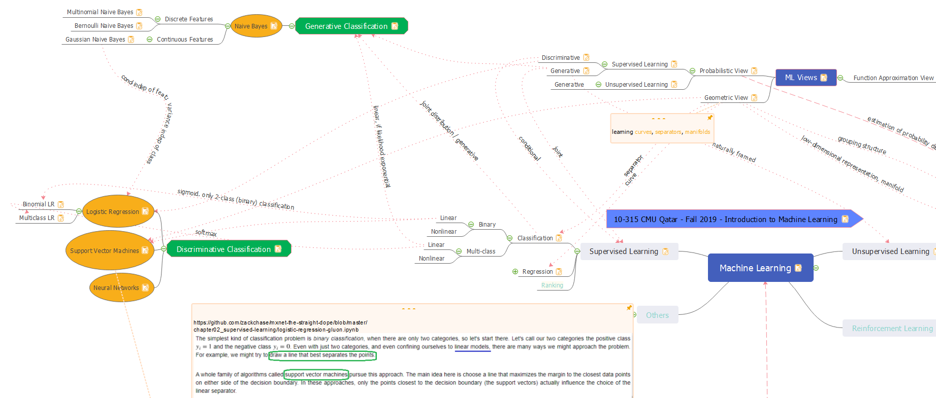
Taxonomy
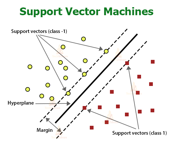
SVM is not probabilistic. SVM takes a geometric approach to classification. It is a discriminative classifier. It is a binary classification algorithm. The classifier finds a linear hyperplane separating the two classes of data points. It is parametric, with weights and a bias for the features, and lagrange multipliers for the constraints.
Multi-class SVM can be developed using a one-vs-one or a one-vs-all approach.
In summary, a SVM classifier is:
- Non-Probabilistic, Geometric
- Discriminative
- Binary
- Linear
- Parametric
Imports
import numpy as np #arrays for data points
from numpy.random import normal, randint #gaussian distributed data points
from numpy import dot #vector dot product for the linear kernel
import pandas as pd #create dataframe from data points, for plotting using sns
import matplotlib.pyplot as plt #plotting
import seaborn as sns #plotting
%matplotlib inline
X_m, Y
Data Configuration
M = 100 #number of data points
n_features = 2 #number of dimensions
cols = ['X1', 'X2', 'Y'] #column names of the dataframe
K = 2 #number of classes
loc_scale = [(5, 1), (8, 1)] #mean and std of data points belonging to each class
Generate Data
Gaussian clusters in 2D numpy arrays
def generate_X_m_and_Y(M, K, n_features, loc_scale):
    #X_m, Y
    X_m = np.empty((K, (int)(M/2), n_features), dtype=float) #initialize data points
    Y = np.empty((K, (int)(M/2)), dtype=int) #initialize the class labels
    for k in range(K): #for each class, generate data points #create data points for each class
        #create data points for class k using gaussian (normal) distribution
        X_m[k] = normal(loc=loc_scale[k][0], scale=loc_scale[k][1], size=((int)(M/2), n_features))
        #create labels (-1, +1) for class k (0, 1).
        #trick: for k=0, label is -1+2*0=-1; for k=1, label is -1+2*1=1
        Y[k] = np.full(((int)(M/2)), -1 + 2*k, dtype=int)
    X_m = X_m.reshape(M, K) #collapse the class axis
    Y = Y.reshape(M) #collapse the class axis
    X_m.shape, Y.shape #print shapes

    return X_m, Y

X_m, Y = generate_X_m_and_Y(M, K, n_features, loc_scale)
X_m, Y in DataFrame
def create_df_from_array(X_m, Y, n_features, cols):
    #create series from each column of X_m, and a series from Y
    l_series = [] #list of series, one for each column
    for feat in range(n_features): #create series from each column of X_m
        l_series.append(pd.Series(X_m[:, feat])) #create series from a column of X_m
    l_series.append(pd.Series(Y[:])) #create series from Y

    frame = {col : series for col, series in zip(cols, l_series)} #map of column names to series
    df = pd.DataFrame(frame) #create dataframe from map

    return df

df = create_df_from_array(X_m, Y, n_features, cols)
df.sample(n = 10)
| X1 | X2 | Y | |
|---|---|---|---|
| 40 | 5.211933 | 3.162270 | -1 |
| 96 | 7.682917 | 9.953946 | 1 |
| 22 | 2.870566 | 5.851050 | -1 |
| 43 | 3.325478 | 3.798079 | -1 |
| 59 | 7.752266 | 8.119911 | 1 |
| 52 | 7.489131 | 8.838146 | 1 |
| 2 | 4.896474 | 4.321929 | -1 |
| 57 | 10.056611 | 7.791627 | 1 |
| 84 | 8.746390 | 7.573401 | 1 |
| 32 | 5.165944 | 5.219445 | -1 |
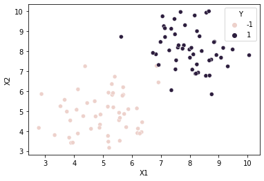
#scatter plot of data points
#class column Y is passed in as hue
sns.scatterplot(x=cols[0], y=cols[1], hue=cols[2], data=df)
<AxesSubplot:xlabel='X1', ylabel='X2'>
Model
Model Configuration
#cost to pay if functional margin is < 1
C = 0.6 #regularization parameter

#tolerance for meeting the KKT conditions that are used to check for convergence
tol = 0.001 #tolerance

#number of iterations to perform after the alphas have converged
max_passes = 5
Model Prediction Data Structures
Note that alphas and bias are created here for testing the functions that follow. They will be created fresh inside the SMO algorithm.
#estimated lagrangian Multipliers
#most of the alphas will be close to zero, except for alphas of data points that are support vectors
alphas = np.zeros((M), dtype=float) #one multiplier for each data point

#bias of the dual problem
#in the primal problem, we have both w (weights) and b (bias).
#in the dual problem, w is replaced with alpha, but b remains.
bias = 0.0
Linear Kernel
'''linear kernel : compute the dot product of the 2 vectors

    returns:
        (float) the dot product of the 2 vectors

    parameters:
        X1: the first vector
        X2: the second vector
'''
def k_lin(X1, X2):
    return dot(X1, X2)
Predict (eq 2)
'''predict the label given the input, training data, and learnt parameters alphas and bias.
    this is equivalent to WX + b, but using alphas instead of W.
'''
def fx(X, X_m, Y, alphas, bias, knl = k_lin):
    pred = 0.0
    for i, Xi in enumerate(X_m):
        pred += alphas[i] * Y[i] * knl(Xi, X)

    return pred + bias

fx(X_m[0], X_m, Y, alphas, bias)
0.0
Error for a data point (eq 13)
'''error between the SVM output and the true label
'''
def Err(X, y, X_m, Y, alphas, bias, knl = k_lin):
    #predict the label
    y_pred = fx(X, X_m, Y, alphas, bias, knl)

    return y_pred - (float)(y)

Err(X_m[0], Y[0], X_m, Y, alphas, bias)
1.0
KKT Dual Complementarity Conditions (eq 6-8)
The above equations translate into the following pseudo-code:

'''Karush-Kuhn-Tucker conditions
'''
def kkt(y, err, alpha):
    if ((y * err < -tol) and (alpha < C)) or \
    ((y * err > tol) and (alpha > 0)):
        return True

    return False

err = Err(X_m[0], Y[0], X_m, Y, alphas, bias)
kkt(Y[0], err, alphas[0])
True
L and H - boundary constraints on alphas (eq 10-11)
def LH(yi, yj, ai, aj):
    if yi != yj:
        L, H = max(0, aj-ai), min(C, C+aj-ai)
    else:
        L, H = max(0, ai+aj-C), min(C, ai+aj)

    #if(L > H):
        #print('L IS GREATER THAN H: L=', L, ' H=', H, ' yi=', yi, ' yj=', yj, ' ai=', ai, ' aj=', aj)

    return L, H

LH(Y[0], Y[1], alphas[0], alphas[1])
(0, 0.0)
n - denominator when calculating optimal alpha_j (eq 14)
'''denominator when calculating optimal alpha_j
'''
def n_den(Xi, Xj, knl = k_lin):
    return 2 * knl(Xi, Xj) - knl(Xi, Xi) - knl(Xj, Xj) #TODO line 63 return (-1) *

n_den(X_m[0], X_m[1])
-1.6061731002951376
alpha_j (eq 12)
def alpha_j(aj, yj, err_i, err_j, n):
    return aj - ((yj * (err_i - err_j)) / n) #TODO line 65 aj +

i, j = 0, M-1
Xi, Xj, Yi, Yj = X_m[i], X_m[j], Y[i], Y[j]
err_i = Err(Xi, Yi, X_m, Y, alphas, bias)
err_j = Err(Xj, Yj, X_m, Y, alphas, bias)
n = n_den(Xi, Xj)
aj = alpha_j(alphas[j], Yj, err_i, err_j, n)
print('Xi=', Xi, 'Yi=', Yi)
print('Xj=', Xj, 'Yj=', Yj)
print('err_i=', err_i, 'err_j=', err_j, 'n=', n, 'aj=', aj)
Xi= [2.7774898  4.15832218] Yi= -1
Xj= [6.98985299 8.45370087] Yj= 1
err_i= 1.0 err_j= -1.0 n= -36.19428180189391 aj= 0.05525734730548922
clipped / constrained alpha_j (eq 15)
def clip_alpha_j(aj, L, H):
    if aj > H:
        return H
    elif (L <= aj and aj <= H):
        return aj
    else:
        return L

i, j = 0, M-1
Xi, Xj, Yi, Yj = X_m[i], X_m[j], Y[i], Y[j]
err_i = Err(Xi, Yi, X_m, Y, alphas, bias)
err_j = Err(Xj, Yj, X_m, Y, alphas, bias)
n = n_den(Xi, Xj)
aj = alpha_j(alphas[j], Yj, err_i, err_j, n)
print('aj_old=', alphas[j], 'aj_new=', aj)
L, H = LH(Y[i], Y[j], alphas[i], aj)
aj = clip_alpha_j(aj, L, H)
print('L=', L, 'H=', H, 'aj_clipped=', aj)
aj_old= 0.0 aj_new= 0.05525734730548922
L= 0.05525734730548922 H= 0.6 aj_clipped= 0.05525734730548922
alpha_i (eq 16)
def alpha_i(ai, aj_old, aj, yi, yj):
    return ai + (yi * yj * (aj_old - aj))

i, j = 0, M-1
Xi, Xj, Yi, Yj = X_m[i], X_m[j], Y[i], Y[j]
err_i = Err(Xi, Yi, X_m, Y, alphas, bias)
err_j = Err(Xj, Yj, X_m, Y, alphas, bias)
n = n_den(Xi, Xj)
aj = alpha_j(alphas[j], Yj, err_i, err_j, n)
print('aj_old=', alphas[j], 'aj_new=', aj)
L, H = LH(Y[i], Y[j], alphas[i], aj)
aj = clip_alpha_j(aj, L, H)
print('L=', L, 'H=', H, 'aj_clipped=', aj)
ai = alpha_i(alphas[i], alphas[j], aj, Yi, Yj)
print('ai_old=', alphas[i], 'ai_new=', ai)
aj_old= 0.0 aj_new= 0.05525734730548922
L= 0.05525734730548922 H= 0.6 aj_clipped= 0.05525734730548922
ai_old= 0.0 ai_new= 0.05525734730548922
b1, b2, b (eq 17-19)
def b1(Xi, Xj, Yi, Yj, ai_old, ai, aj_old, aj, b, err_i, knl = k_lin):
    return b - err_i - Yi * (ai - ai_old) * knl(Xi, Xi) - Yj * (aj - aj_old) * knl(Xi, Xj)
def b2(Xi, Xj, Yi, Yj, ai_old, ai, aj_old, aj, b, err_j, knl = k_lin):
    return b - err_j - Yi * (ai - ai_old) * knl(Xi, Xj) - Yj * (aj - aj_old) * knl(Xj, Xj)
def b(b1, b2, ai, aj):
    if (ai > 0 and ai < C):
        return b1
    elif (aj > 0 and aj < C):
        return b2
    else:
        return (b1 + b2)/2
i, j = 0, M-1
Xi, Xj, Yi, Yj = X_m[i], X_m[j], Y[i], Y[j]
err_i = Err(Xi, Yi, X_m, Y, alphas, bias)
err_j = Err(Xj, Yj, X_m, Y, alphas, bias)
n = n_den(Xi, Xj)
ai_old = alphas[i]
aj_old = alphas[j]
aj = alpha_j(aj_old, Yj, err_i, err_j, n)
print('aj_old=', aj_old, 'aj_new=', aj)
L, H = LH(Y[i], Y[j], ai_old, aj)
aj = clip_alpha_j(aj, L, H)
print('L=', L, 'H=', H, 'aj_clipped=', aj)
ai = alpha_i(ai_old, aj_old, aj, Yi, Yj)
print('ai_old=', ai_old, 'ai_new=', ai)

b1_val = b1(Xi, Xj, Yi, Yj, ai_old, ai, aj_old, aj, bias, err_i)
print('b1=', b1_val)
b2_val = b2(Xi, Xj, Yi, Yj, ai_old, ai, aj_old, aj, bias, err_j)
print('b2=', b2_val)
b_val = b(b1_val, b2_val, ai, aj)
print('b=', b_val)
aj_old= 0.0 aj_new= 0.05525734730548922
L= 0.05525734730548922 H= 0.6 aj_clipped= 0.05525734730548922
ai_old= 0.0 ai_new= 0.05525734730548922
b1= -2.6334825719646275
b2= -2.6334825719646275
b= -2.6334825719646275
select random j
#select a j not equal to i
def sel_rand_j(i):
    j = randint(M) #select a random number j in the range 0..M-1
    while (j==i): #while we got i as the random number, in which case j == i, we keep trying a different random number
        j = randint(M) #try a different random number
    return j #now we have a random number in the range 0..M that is not equal to i
Simplified SMO
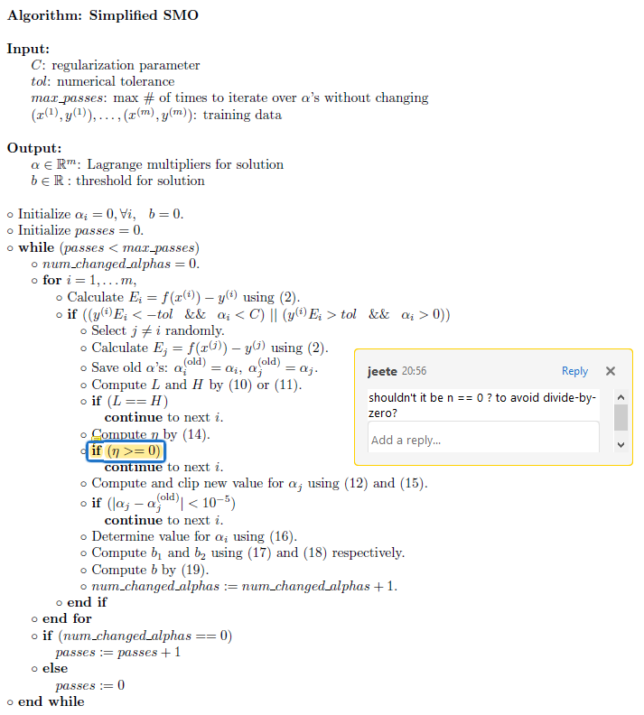
pseudo-code
python code
def simplified_smo(C, tol, max_passes, X_m, Y, knl = k_lin):

    #1 Initialize alphas, and beta

    #estimated lagrangian Multipliers
    #most of the alphas will be close to zero, except for alphas of data points that are support vectors
    a_m = np.zeros((M), dtype=float) #one multiplier for each data point

    #bias of the dual problem
    #in the primal problem, we have both w (weights) and b (bias).
    #in the dual problem, w is replaced with alpha, but b remains.
    b_val = 0.0

    #2 count number of passes after the alphas have converged
    passes = 0

    #3 while alphas are converging, and a little beyond (max_passes beyond convergence)
    while (passes < max_passes):
        #3.1 number of alphas that changed.
        #    if they are greater than zero, we reset passes to 0. (alphas have not converged yet)
        #    if they are equal to zero, we increment passes up to max_passes, allowing alphas to converge further if they can.
        num_changed_alphas = 0

        #3.2 loop over the dataset, trying to converge 2 alphas
        for i in range(M):

            #3.2.1 calculate error between predicted label and actual label for data point i
            err_i = Err(X_m[i], Y[i], X_m, Y, a_m, b_val, knl)

            #3.2.2 if the KKT conditions are met
            if (kkt(Y[i], err_i, a_m[i])):
                #3.2.2.1 select j != i randomly
                j = sel_rand_j(i)
                #3.2.2.2 calculate error between predicted label and actual label for data point j
                err_j = Err(X_m[j], Y[j], X_m, Y, a_m, b_val, knl)
                #3.2.2.3 save old alphas
                ai_old, aj_old = a_m[i], a_m[j]
                #3.2.2.4 compute L and H
                L, H = LH(Y[i], Y[j], a_m[i], a_m[j])
                #3.2.2.5 if L and H are the same, we try again with a different alpha_i
                if (L == H):
                    continue
                #3.2.2.6 compute the denominator n
                n = n_den(X_m[i], X_m[j], knl)
                #3.2.2.7 if n == 0, we treat this as a case where we cannot make progress on this pair of alphas
                if (n == 0):#TODO n==0 or > =0
                    continue
                #3.2.2.8 compute and clip the new value of alpha_j
                a_m[j] = alpha_j(a_m[j], Y[j], err_i, err_j, n)
                a_m[j] = clip_alpha_j(a_m[j], L, H)
                #3.2.2.9 if alpha_j has converged, move to a new set of alphas
                if abs(a_m[j] - aj_old) < pow(10, -5): #has alpha_j converged? #TODO abs
                    continue
                #3.2.2.10 determine value of alpha_i
                a_m[i] = alpha_i(ai_old, aj_old, a_m[j], Y[i], Y[j]) # ai = ai + yi*yj*(aj_old - aj)
                #3.2.2.11 compute b1 and b2
                b1_val = b1(X_m[i], X_m[j], Y[i], Y[j], ai_old, a_m[i], aj_old, a_m[j], b_val, err_i)
                b2_val = b2(X_m[i], X_m[j], Y[i], Y[j], ai_old, a_m[i], aj_old, a_m[j], b_val, err_j)
                #3.2.2.12 compute b
                b_val = b(b1_val, b2_val, a_m[i], a_m[j])
                #3.2.2.13 increment the number of alphas changed
                num_changed_alphas += 1
            #end if 3.2.2
        #end for 3.2

        #3.3 if no alphas changed, increment passes a little beyond convergence
        if (num_changed_alphas == 0):
            passes += 1
        else: #some alphas changed, so we reset passes
              # and start incrementing num_changed_alphas again when alphas begin to converge
            passes = 0

        print('Number of lagrange multipliers still converging:', num_changed_alphas)

    #end while 3

    #return the converged alphas (lagrange multipliers), and the threshold (beta) for the solution
    return a_m, b_val
Learn
a_m, b_val = simplified_smo(C, tol, max_passes, X_m, Y)
Number of lagrange multipliers still converging: 7
Number of lagrange multipliers still converging: 6
Number of lagrange multipliers still converging: 3
Number of lagrange multipliers still converging: 6
Number of lagrange multipliers still converging: 8
Number of lagrange multipliers still converging: 4
Number of lagrange multipliers still converging: 1
Number of lagrange multipliers still converging: 1
Number of lagrange multipliers still converging: 2
Number of lagrange multipliers still converging: 0
Number of lagrange multipliers still converging: 0
Number of lagrange multipliers still converging: 0
Number of lagrange multipliers still converging: 3
Number of lagrange multipliers still converging: 1
Number of lagrange multipliers still converging: 2
Number of lagrange multipliers still converging: 2
Number of lagrange multipliers still converging: 2
Number of lagrange multipliers still converging: 2
Number of lagrange multipliers still converging: 0
Number of lagrange multipliers still converging: 2
Number of lagrange multipliers still converging: 2
Number of lagrange multipliers still converging: 0
Number of lagrange multipliers still converging: 0
Number of lagrange multipliers still converging: 1
Number of lagrange multipliers still converging: 1
Number of lagrange multipliers still converging: 4
Number of lagrange multipliers still converging: 2
Number of lagrange multipliers still converging: 0
Number of lagrange multipliers still converging: 1
Number of lagrange multipliers still converging: 3
Number of lagrange multipliers still converging: 2
Number of lagrange multipliers still converging: 1
Number of lagrange multipliers still converging: 0
Number of lagrange multipliers still converging: 1
Number of lagrange multipliers still converging: 1
Number of lagrange multipliers still converging: 1
Number of lagrange multipliers still converging: 1
Number of lagrange multipliers still converging: 1
Number of lagrange multipliers still converging: 0
Number of lagrange multipliers still converging: 0
Number of lagrange multipliers still converging: 0
Number of lagrange multipliers still converging: 0
Number of lagrange multipliers still converging: 0
Support Vectors
#support vectors information
sv_ind = np.nonzero(a_m) #alpha indices
sv_a_m = a_m[sv_ind] #alphas
sv_X_m = X_m[sv_ind] #vectors
sv_Y = Y[sv_ind] #class

print('Number of Support Vectors:', len(sv_a_m))
print('Support Vectors:\n', sv_X_m)
print('Alphas:\n', sv_a_m)
Number of Support Vectors: 12
Support Vectors:
 [[4.01672464 4.95910969]
 [4.58939644 6.24781842]
 [6.42969753 4.23687801]
 [3.35352254 4.06678074]
 [5.29936958 3.58851751]
 [9.47171399 8.02614293]
 [7.07618927 7.11401766]
 [7.76384263 7.68750358]
 [6.44359498 6.87073672]
 [5.55611474 7.46208598]
 [6.86536742 9.13082197]
 [6.66468045 8.32477016]]
Alphas:
 [0.10383806 0.6        0.6        0.02436853 0.50294886 0.15664808
 0.35682867 0.6        0.03845793 0.40089538 0.16180494 0.11652045]
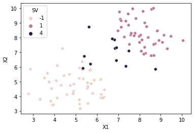
Plot the Support vectors
#color/hue of support vectors is
sv_hue = 4 #some value other than -1, +1 used for class labels
svecs = [y if ai == 0 else sv_hue for ai, y in zip(a_m, df['Y'].to_list())]
df['SV'] = svecs

#scatter plot of data points
#class column Y is passed in as hue
sns.scatterplot(x=cols[0], y=cols[1], hue='SV', data=df)
<AxesSubplot:xlabel='X1', ylabel='X2'>
Prediction
Generate Data
Gaussian clusters in 2D numpy arrays
X_m, Y = generate_X_m_and_Y(M, K, n_features, loc_scale) #generate test data points
Predict
Y_pred = [fx(X_m[i], sv_X_m, sv_Y, sv_a_m, b_val) for i in range(M)] #predict (margin of) testing data
Y_pred_class = [-1 if y < 0 else 1 for y in Y_pred] #decision based on predicted margin
Predicted X_m, Y in DataFrame
df = create_df_from_array(X_m, Y, n_features, cols) #create test dataframe
df['Y_pred_margin'] = Y_pred #append the prediction margin column
df['Y_pred_class'] = Y_pred_class #append the class
df.sample(n = 10)
| X1 | X2 | Y | Y_pred_margin | Y_pred_class | |
|---|---|---|---|---|---|
| 59 | 7.878629 | 8.481838 | 1 | 2.833952 | 1 |
| 20 | 5.884862 | 4.078395 | -1 | -2.751176 | -1 |
| 68 | 9.831908 | 10.121277 | 1 | 5.895153 | 1 |
| 57 | 7.449198 | 7.206902 | 1 | 1.336733 | 1 |
| 81 | 6.443595 | 6.870737 | 1 | 0.218461 | 1 |
| 24 | 4.582161 | 4.861206 | -1 | -3.101826 | -1 |
| 65 | 7.291804 | 8.876164 | 1 | 2.713573 | 1 |
| 1 | 5.773598 | 6.060365 | -1 | -1.055102 | -1 |
| 8 | 3.778248 | 4.542449 | -1 | -4.040887 | -1 |
| 51 | 8.768240 | 8.190470 | 1 | 3.292608 | 1 |
#scatter plot of data points
#class column Y is passed in as hue
sns.scatterplot(x=cols[0], y=cols[1], hue='Y_pred_class', data=df)
<AxesSubplot:xlabel='X1', ylabel='X2'>
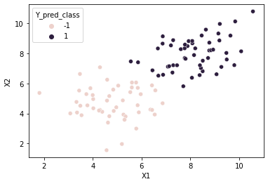
Prediction Accuracy
Y_pred_corr = (Y==Y_pred_class)
num_corr = len(Y_pred_corr[Y_pred_corr == True])
print('Accuracy:', (num_corr/M)*100, '%')
Accuracy: 98.0 %
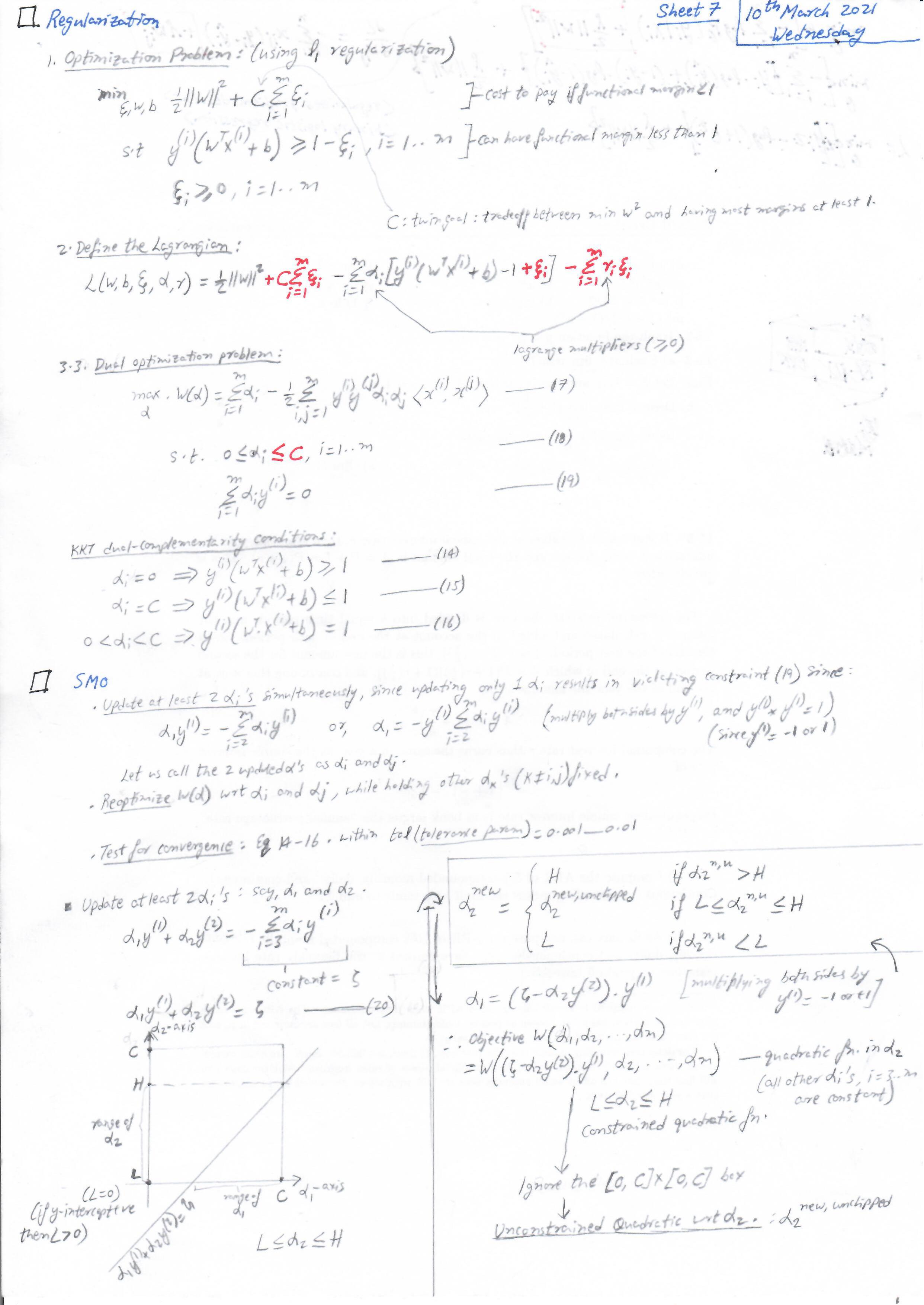
Sidebar - Primal to Dual Problem
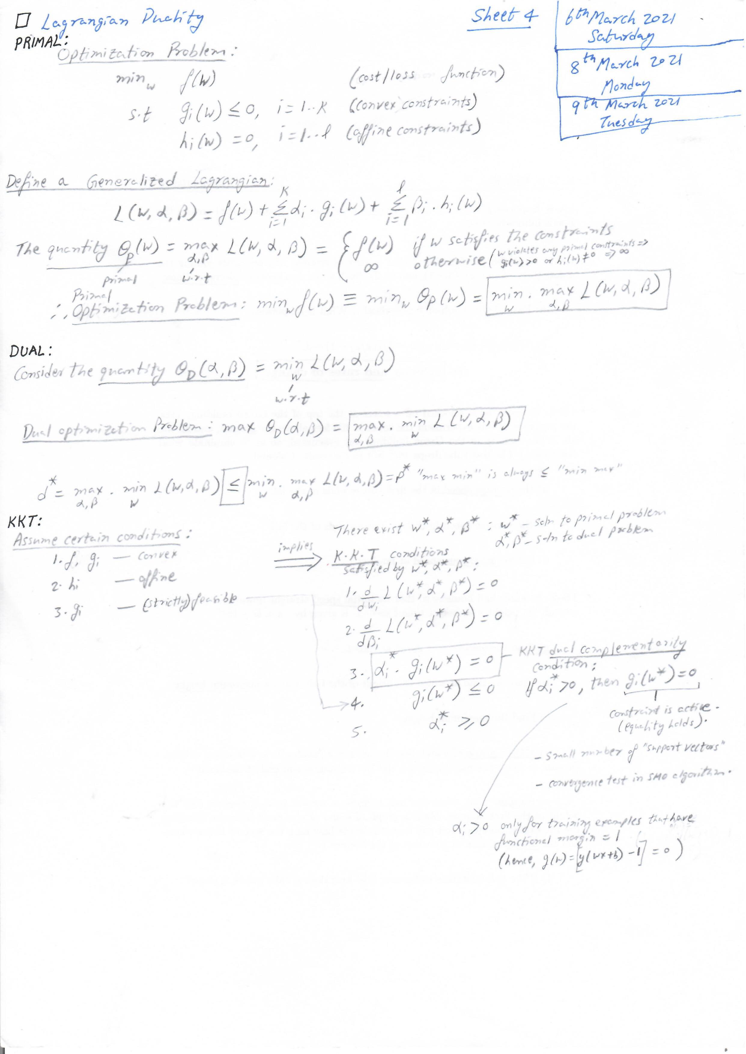
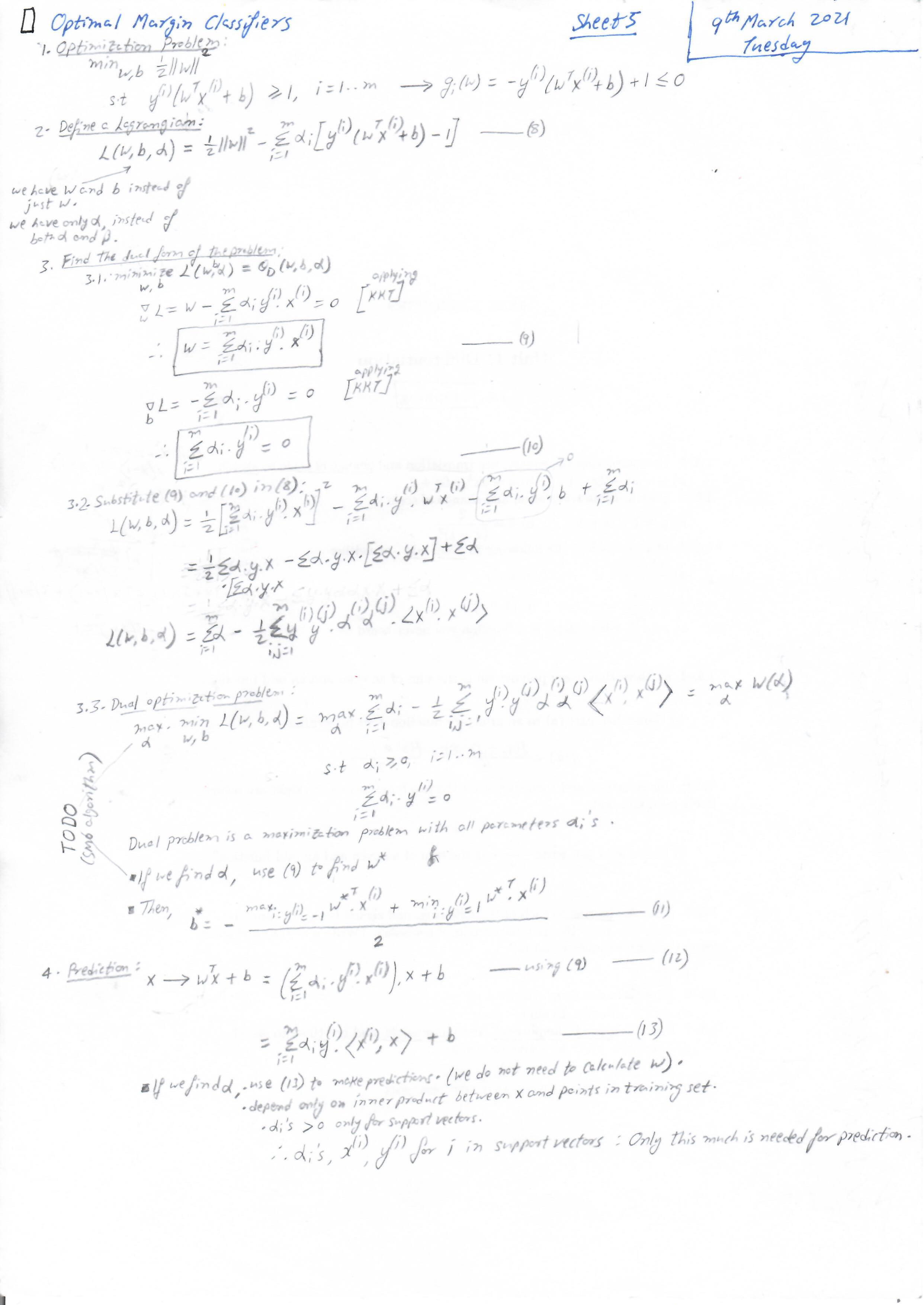
Converting non-convex primal problem to convex dual problem with affine constraints, and then to convex dual problem with no constraints using Lagrange Multipliers.
Refer CS229 notes while understanding my notes below.
- Stanford CS229 Course Notes on SVM
- URL: http://cs229.stanford.edu/summer2020/cs229-notes3.pdf
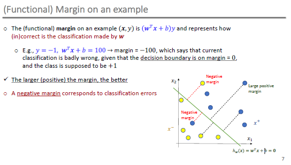
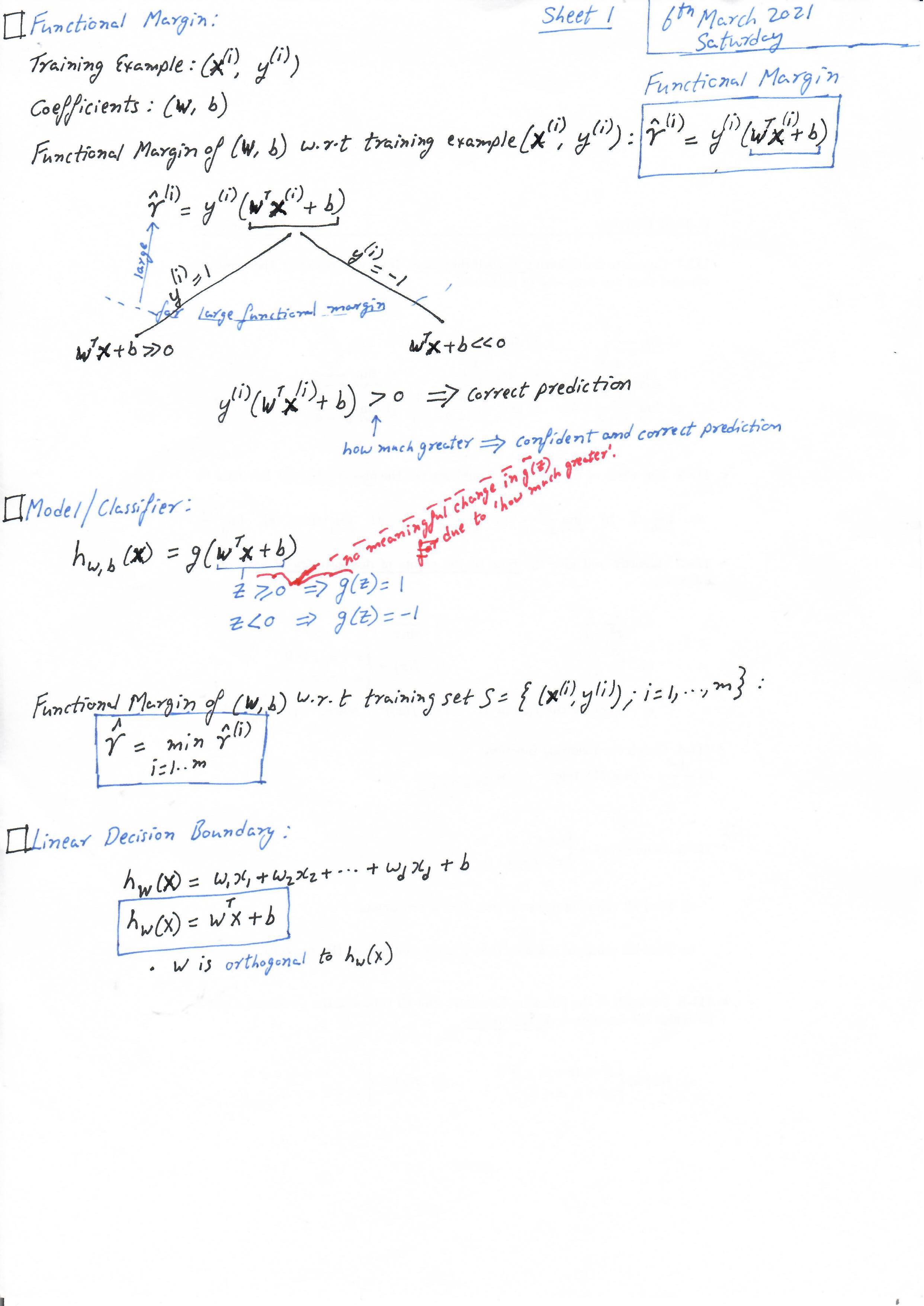
Functional Margin
-
10-315 CMU Qatar
- Fall 2019 - Introduction to Machine Learning
- https://web2.qatar.cmu.edu/~gdicaro/10315/lectures/315-F19-14-SVM-1.pdf
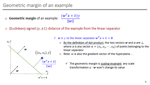
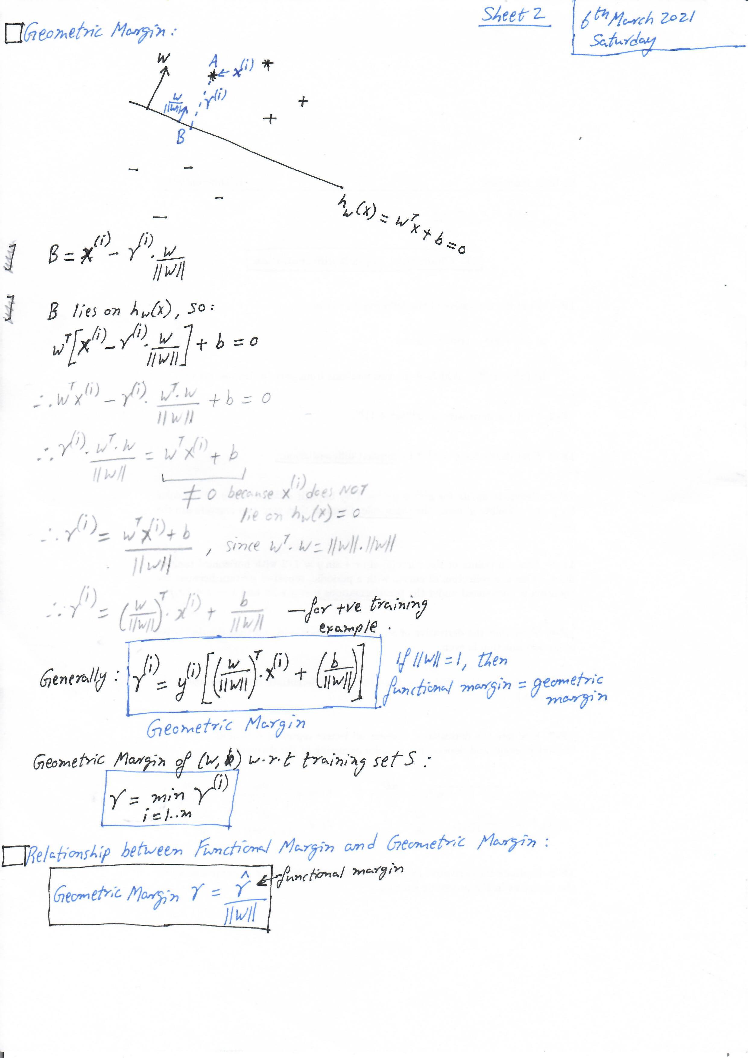
Geometric Margin
Optimization Problem
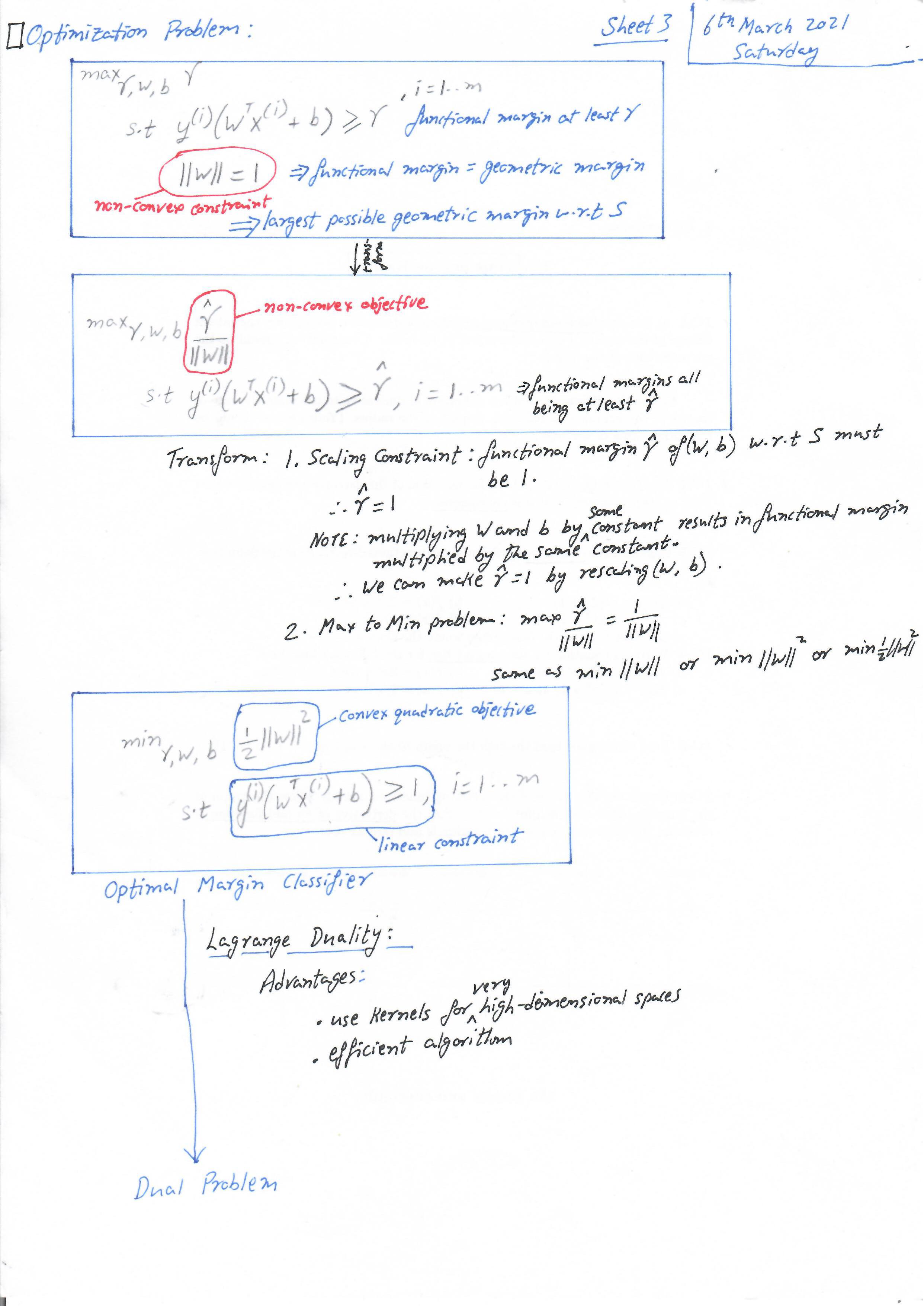
Lagrangian Duality
Optimal Margin Classifiers
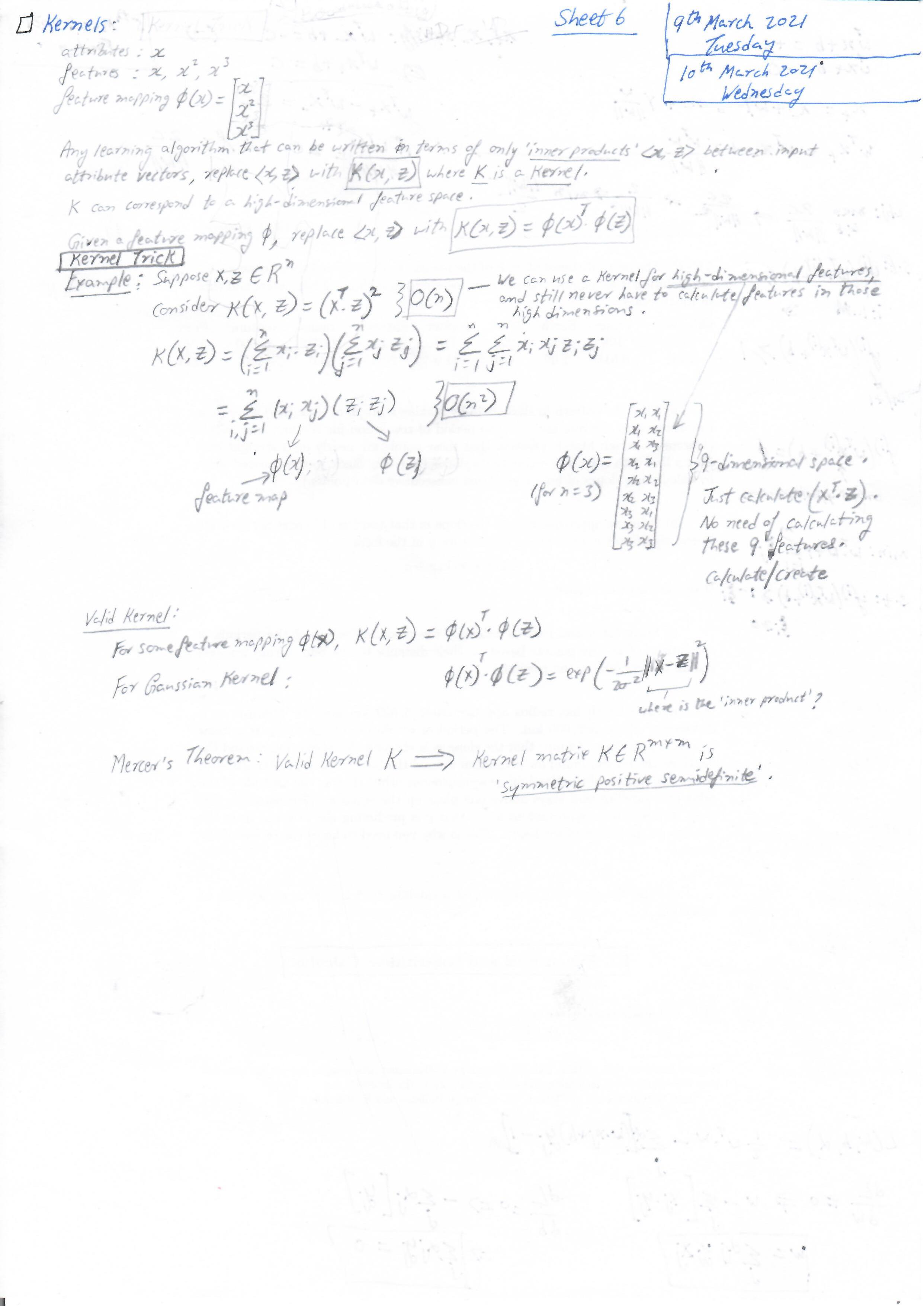
Kernels
Regularization, and SMO