[without library] Iris Flower Species Classification using Multiclass Logistic Regression

Based on - Stanford CS231n - Softmax classifier - Andrej Karpathy, and Cross Entropy Loss Derivative - Roei Bahumi

Introduction

This notebook implements Multinomial Logistic Regression. It performs multi-class classification on Iris Flower Species dataset consisting of four attributes and belonging to three classes. There are 300 data points that we divide into training and test data. The prediction accuracy is 94-100%.

Resources:

Towards the end, I have included a sidebar on the Multinomial Logistic Regression.

Taxonomy and Notes

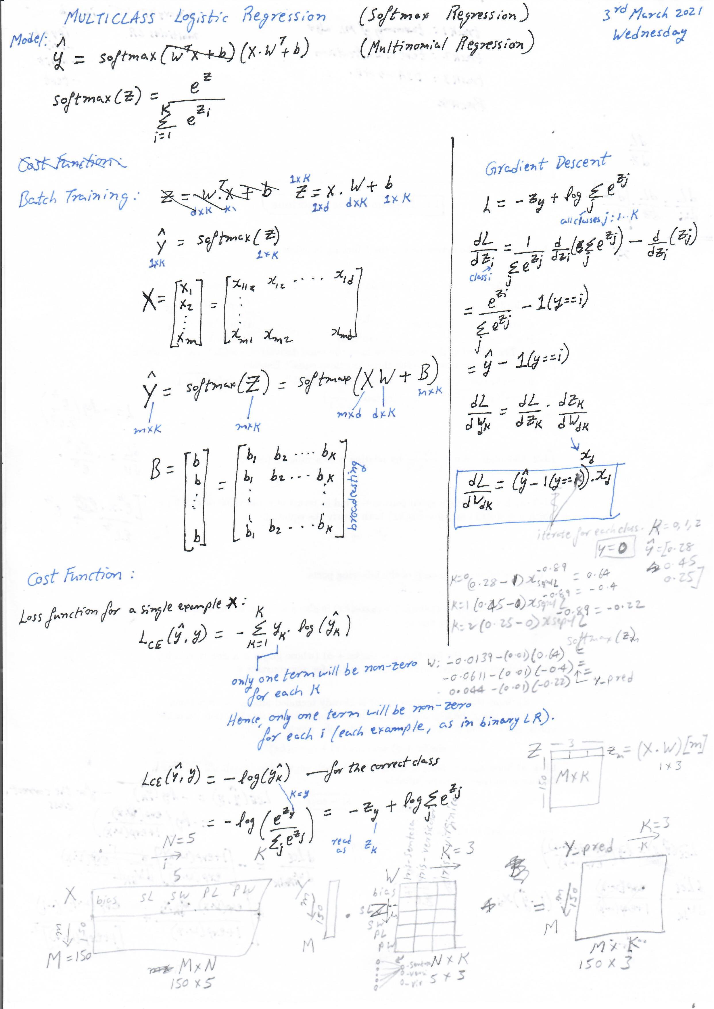
Logistic Regression is a probabilistic classifier. But, it does not model the complete distribution P(X, Y). It is only interested in discriminating among classes. It does that by computing P(Y | X) directly from the training data. Hence, it is a probabilistic-discriminative classifier.

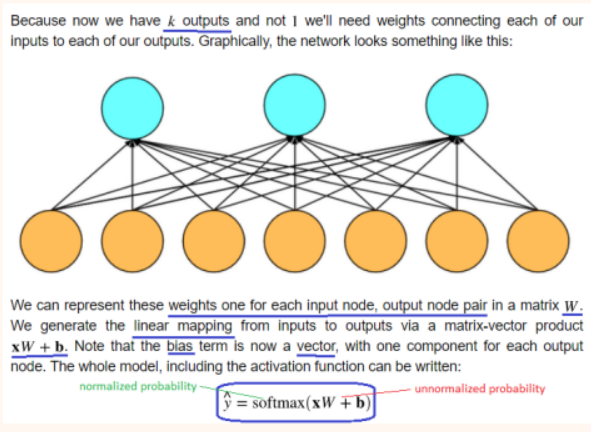
Multinomial Logistic Regression is a composition of K linear functions (K is the number of classes) and the softmax function. Softmax is a generalization of the logistic function to multiple dimensions. It transforms an N-dimensional feature space to a K-dimensional class space. In the case of Iris Flower Species, the N=5 features (bias + sepal/petal length/width) are mapped to K=3 classes. The weight matrix is (N x K), where each column is a linear operator w applied on feature vector x.

It is parametric (weights and bias are the parameters). Binomial Logistic Regression is binary. The model can be modified to use softmax instead of sigmoid, and it becomes Multiclass Logistic Regression.

In summary, Multinomial Logistic Regression is:

Probabilistic
Discriminative
Binary and Multiclass
Linear
Parametric

Imports

import numpy as np
import pandas as pd #input
from numpy.random import rand, normal, standard_normal
from numpy import dot, exp
from numpy import mean, std #mean and standard deviation for gaussian probabilities
from scipy.stats import norm #gaussian probabilities
from math import log # to calculate posterior probability
import matplotlib.pyplot as plt
import seaborn as sns

Data

Data Configuration (1 of 2)

Iris Flower Species

f_data = '../input/iris-species/Iris.csv'
f_cols = ['SepalLengthCm',  'SepalWidthCm',  'PetalLengthCm',  'PetalWidthCm', 'Species']
class_colname = 'Species'

Read

read the csv file

#read the csv file
df = pd.read_csv(f_data)

drop unwanted columns

#drop unwanted columns
drop_cols = list(set(df.columns) - set(f_cols))
df = df.drop(drop_cols, axis = 1)

rename last column that supposedly has a class/label

#rename the last column to 'class'
cols = df.columns.to_list()
cols[len(cols)-1] = class_colname
df.columns = cols

sanity check for data getting loaded

df.sample(5)

	SepalLengthCm	SepalWidthCm	PetalLengthCm	PetalWidthCm	Species
75	6.6	3.0	4.4	1.4	Iris-versicolor
132	6.4	2.8	5.6	2.2	Iris-virginica
89	5.5	2.5	4.0	1.3	Iris-versicolor
35	5.0	3.2	1.2	0.2	Iris-setosa
103	6.3	2.9	5.6	1.8	Iris-virginica

Data Preprocessing

Helper Functions

visualize

def plot_features_violin(data):
    plt.figure(figsize=(15,10))
    plt.subplot(2,2,1)
    sns.violinplot(data=data, x='Species',y='PetalLengthCm')
    plt.subplot(2,2,2)
    sns.violinplot(data=data, x='Species',y='PetalWidthCm')
    plt.subplot(2,2,3)
    sns.violinplot(data=data, x='Species',y='SepalLengthCm')
    plt.subplot(2,2,4)
    sns.violinplot(data=data, x='Species',y='SepalWidthCm')

normalize

'''normalize the features
    
    return:
        copy of the passed in (dataframe), but now with normalized values
        
    parameters:
        df: (dataframe) to normalize
        cols: (list) of columns to normalize
'''
def normalize(df, cols):
    df2 = df.copy(deep = True)
    for col in cols:
        mu = df2[col].mean()
        sigma = df2[col].std()
        df2[col] = (df2[col] - mu) / sigma
        
    return df2

Normalize

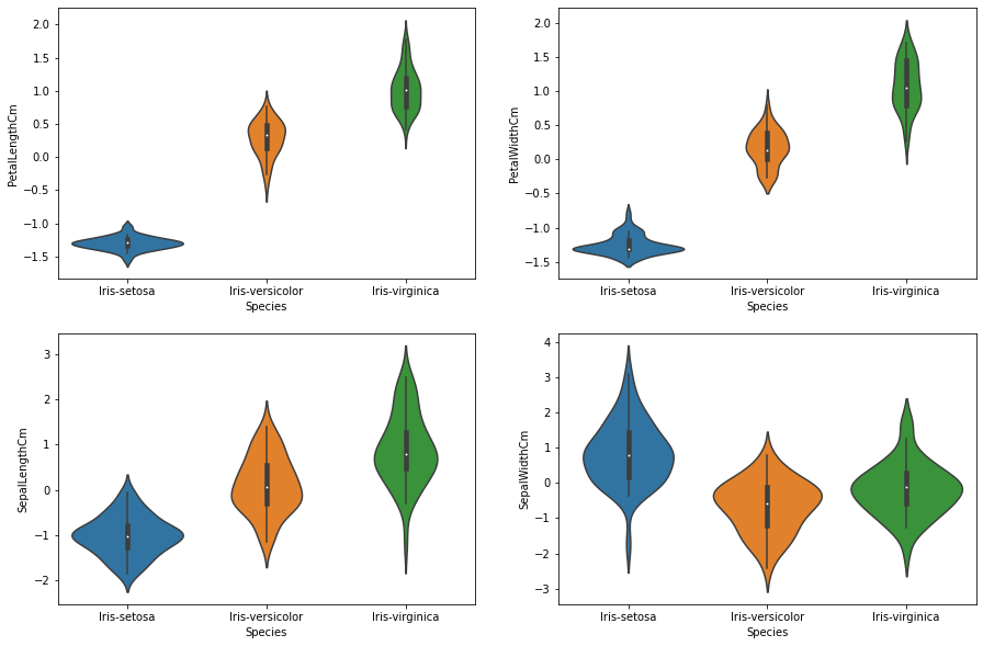
print('Before normalization:\n')
plot_features_violin(df)

Before normalization:

png

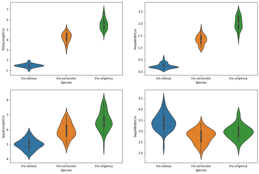
print('\n\nAfter normalization: The relative distribution is still maintained,\
 though the range of values is around 0. (see y-axis markers)\n')
df_norm = normalize(df, f_cols[:-1])
plot_features_violin(df_norm)

After normalization: The relative distribution is still maintained, though the range of values is around 0. (see y-axis markers)

png

Data Configuration (2 of 2)

M: number of data points; N: number of features; K: number of classes

#number of data points, number of attributes
M, N = df_norm.shape[0], df_norm.shape[1]
#number of classes
K = len(df_norm[class_colname].unique())
M, N, K

(150, 5, 3)

Class Names

C = df_norm[class_colname].unique()
C

array(['Iris-setosa', 'Iris-versicolor', 'Iris-virginica'], dtype=object)

X_mn, Y

X_mn

The data points matrix X_mn is a M x N matrix, M being the number of data points, N being the number of attributes

#X_mn: first column is the first input '1' for bias
X_mn = np.ones((M, N), dtype=float)
X_mn[:, 1:] = df_norm.loc[:, df_norm.columns != class_colname].to_numpy()
X_mn.shape

(150, 5)

Y

#Y: class column
Y = np.array(M, dtype=float)
#encode class name to offset in C: array of class names
Y = [np.where(C == c_name)[0][0] for c_name in (df_norm.loc[:, df_norm.columns == class_colname].to_numpy())]
Y = np.array(Y, dtype=int)
Y.shape

(150,)

Model

Model Configuration

loc, scale = 0, 0.1 #to initialize weights
train_ds_percent = 0.8 #to split data into train and test
alpha = 0.001 #learning rate
diff_loss = 0.0001### Model Configuration

Model Prediction Data Structures

W

The weight matrix is an N x K matrix, N being the number of attributes, and K being the number of classes

#initliaze weights randomly
W_nk = normal(loc = loc, scale = scale, size = (N, K))
W_nk.shape

(5, 3)

Predict

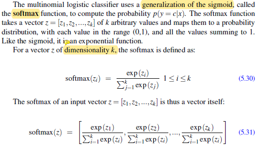
softmax

$q_{i}\left ( z \right )=\frac{e^{z_{i}}}{\sum_{j\in \left \{ 1,..K \right \}}^{}e^{z_{j}}}\; \forall i\in \left \{ 1,..K \right \}$

The equation above shows the softmax calculated for element ‘i’ of the vector Z. Each Z has K elements (K = no. of classes). The function below performs a vector version of softmax, calculating softmax for each element of vector Z and returning the vector of softmax values.

#softmax: normalize each element of Z and return the normalized vector
def softmax_vec(Z):
    # matrix division:
    # numerator: exponentiate each element of Z
    # denominator: exponentiate each element of Z, and then sum them up
    # division: divide each element in the numerator by the sum to normalize it
    return exp(Z) / sum([exp(Z_k) for Z_k in Z])

Y_predicted

#predict K probabilities for each data point in 1..M
# and return a M xK matrix of probabilities
def Y_predicted(X_mn, W_nk):
    Z_mk = dot(X_mn, W_nk)
    #each row Z of Z_mk is passed to softmax to normalize it.
    #Y_pred now has a stack of M normalized Z's.
    #Each Z has K elements (K = no. of classes)
    #so, now, for each data point, we have K probabilities,
    # each telling the probability of the data point belonging to class k = 1..K
    Y_pred = np.stack([softmax_vec(Z) for Z in Z_mk])
    return Y_pred # M x K matrix

Cost (cross-entropy loss)(negative log likelihood loss)

$H\left ( p, q \right )=-\sum_{x}^{}p\left ( x \right )\; log \; q\left ( x \right )$

'''Cross-Entropy Loss

    returns:
        (float) cross-entropy loss from predictions
        
    parameters:
        Y_pred: (M.K array) (numDataPoints.numClasses) predicted class probabilities for M data points
        Y: (M.1 array) (numDataPoints) actual class for M data points
'''
def Loss_ce(Y_pred, Y):
    L_ce = 0.0
    for m, k in enumerate(Y):
        L_ce += (-1)*log(Y_pred[m][k])
    return L_ce

Loss_ce(Y_predicted(X_mn, W_nk), Y)

168.64146013824276

Gradient

$\frac{\partial l\left ( W \right )}{\partial w_{i}}=\sum_{i}^{}X_{i}^{l}\left ( Y^{l}-\hat{P}\left ( Y^{l}=1|X^{l}, W \right ) \right )$

def gradients(X_mn, Y, Y_pred, N, K):
    #gradient along each of the N attributes, for each of the K classes
    grads = np.zeros((N, K), dtype=float)
    for j in range(N):
        for k in range(K):
            for m, X in enumerate(X_mn):
                grads[j][k] += (Y_pred[m][k] - (int)(Y[m]==k))*X[j]

    return grads

gradients(X_mn, Y, Y_predicted(X_mn, W_nk), N, K)

array([[ -0.39155471,   2.19089601,  -1.7993413 ],
       [ 46.39999389,   2.24131206, -48.64130594],
       [-46.75856991,  31.37213789,  15.38643202],
       [ 62.30179774,  -6.00141406, -56.30038368],
       [ 59.5940192 ,  -0.19498116, -59.39903804]])

Training Algorithm

$w_{i}\leftarrow w_{i}+\eta \sum_{l}^{}X_{i}^{l}\left ( Y^{l}-\hat{P}\left ( Y^{l}=1|X^{l}, W \right ) \right )$

def train(X_mn, Y, W_nk):
    Y_pred = Y_predicted(X_mn, W_nk) #predicted probabilities
    prev_loss = Loss_ce(Y_pred, Y) #loss to begin with
    dLdW = gradients(X_mn, Y, Y_pred, N, K) #gradient along each of the N attributes, for each of the K classes
    W_nk = W_nk - (alpha * dLdW) #apply learning_rate*gradient to the weights
    Y_pred = Y_predicted(X_mn, W_nk) #predicted probabilities with new weights
    new_loss = Loss_ce(Y_pred, Y) #predicted probabilities with new weights
    #summary print
    i_print = 0
 
    #while the loss function is still converging rapidly
    while (prev_loss - new_loss > diff_loss):
        if(i_print % 500) == 0:
            print('Cost:', new_loss)
        prev_loss = new_loss #backup the loss to previous loss for convergence detection
        dLdW = gradients(X_mn, Y, Y_pred, N, K) #gradient along each of the N attributes, for each of the K classes
        W_nk = W_nk - (alpha * dLdW) #apply learning_rate*gradient to the weights
        Y_pred = Y_predicted(X_mn, W_nk) #predicted probabilities with new weights
        new_loss = Loss_ce(Y_pred, Y) #predicted probabilities with new weights
        i_print += 1
        
    return W_nk

Learn

Divide data into Train and Test

mask = rand(M) < train_ds_percent
X_tr, Y_tr, X_te, Y_te = X_mn[mask], Y[mask], X_mn[~mask], Y[~mask]
X_tr.shape, Y_tr.shape, X_te.shape, Y_te.shape

((116, 5), (116,), (34, 5), (34,))

Learn

W_nk = train(X_tr, Y_tr, W_nk)

Cost: 116.6483283544849
Cost: 18.249658848820356
Cost: 12.951954448719748
Cost: 10.645191711359773
Cost: 9.324411602909944
Cost: 8.452276659013673
Cost: 7.824010517344139
Cost: 7.344201154723735
Cost: 6.962156632256088
Cost: 6.648325577035544
Cost: 6.384245774778408
Cost: 6.157746375601451
Cost: 5.960451836587583
Cost: 5.786392123110191
Cost: 5.6311851365748495
Cost: 5.491533384283073
Cost: 5.36490201563757
Cost: 5.249306026851437
Cost: 5.14316558536557
Cost: 5.045205207521434
Cost: 4.954381949702238
Cost: 4.8698332639541295
Cost: 4.790838471178479
Cost: 4.716789847874346
Cost: 4.647170618675076
Cost: 4.581537988365074
Cost: 4.519509904618752
Cost: 4.460754619121964
Cost: 4.404982373239275
Cost: 4.351938714714369

Prediction

Predict

Y_pred_k = [np.argmax(y_pred_k) for y_pred_k in Y_predicted(X_te, W_nk)]

Prediction Accuracy

matches = sum([int(pred==actual) for pred, actual in zip(Y_pred_k, Y_te)])
print('Accuracy is', (matches*100)/len(Y_te), 'percent.')

Accuracy is 94.11764705882354 percent.

[without library] Iris Flower Species Classification using Multiclass Logistic Regression

Based on - Stanford CS231n - Softmax classifier - Andrej Karpathy, and Cross Entropy Loss Derivative - Roei Bahumi

Introduction

Taxonomy and Notes

Imports

Data

Data Configuration (1 of 2)

Iris Flower Species

Read

read the csv file

drop unwanted columns

rename last column that supposedly has a class/label

sanity check for data getting loaded

Data Preprocessing

Helper Functions

visualize

normalize

Normalize

Data Configuration (2 of 2)

M: number of data points; N: number of features; K: number of classes

Class Names

X_mn, Y

X_mn

Y

Model

Model Configuration

Model Prediction Data Structures

W

Predict

softmax

Y_predicted

Cost (cross-entropy loss)(negative log likelihood loss)

Gradient

Training Algorithm

Learn

Divide data into Train and Test

Learn

Prediction

Predict

Prediction Accuracy

Sidebar - Multiclass Logistic Regression

Why Softmax?

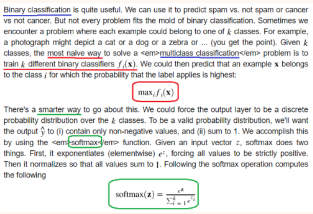
Why linear?

Generalization of sigmoid to softmax

Negative Log-Likelihood Loss

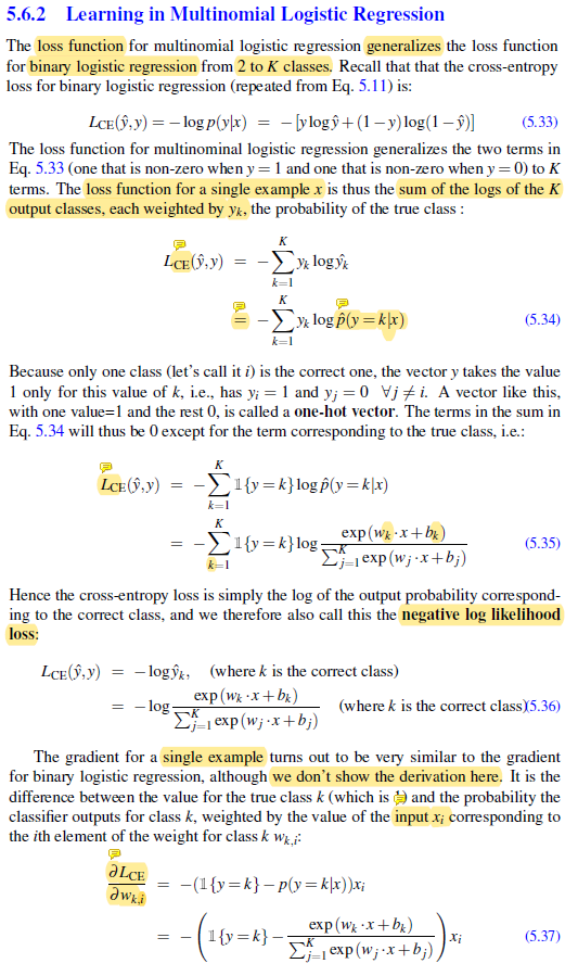
Derivation of Eq.5.37 (gradient for a single example)