[without library] Binary Classification using Logistic Regression
[without library] Binary Classification using Logistic Regression
</font>
Based on - [2010] Generative and Discriminative Classifiers : Naive Bayes and Logistic Regression - Tom Mitchell
Introduction
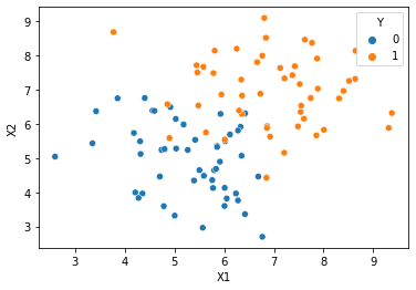
This notebook implements Binomial Logistic Regression. It performs binary classification on a generated dataset consisting of two gaussian distributed clusters of points in a 2-dimensional space. The prediction accuracy for a learning dataset of 100 points is 90+% if the clusters overlap slightly and 98-100% if the clusters do not overlap.
Resources:
Towards the end, I have included a sidebar on the Binomial Logistic Regression.
Taxonomy and Notes
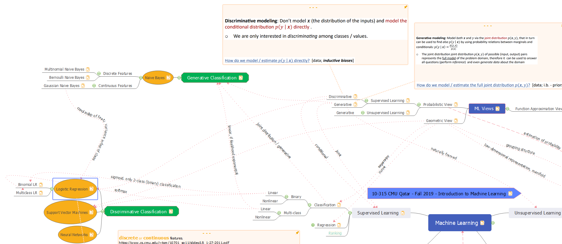
Logistic Regression is a probabilistic classifier. But, it does not model the complete distribution P(X, Y). It is only interested in discriminating among classes. It does that by computing P(Y|X) directly from the training data. Hence, it is a probabilistic-discriminative classifier. The classifier’s sigmoid function is linear in terms of weights and bias for the features. It is parametric (weights and bias are the parameters). Binomial Logistic Regression is binary. The model can be modified to use softmax instead of sigmoid, and it becomes Multiclass Logistic Regression.
In summary, Logistic Regression is:
- Probabilistic
- Discriminative
- Binary and Multiclass
- Linear
- Parametric
The density estimation of P(Y|X) is parametric, point estimation, using Maximum Likelihood Estimation (MLE).
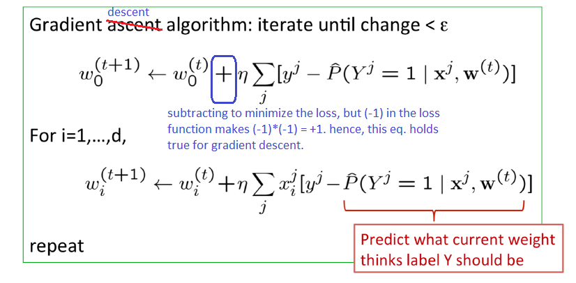
The computation of P(Y|X) is not in closed-form. So, a numerical method like Gradient Descent is used to optimize the model’s cost function.
Imports
from math import log # to calculate posterior probability
import numpy as np #arrays for data points
from numpy.random import rand, normal, randint #gaussian distributed data points
from numpy import dot #vector dot product for the linear kernel
from numpy import mean, std #mean and standard deviation for gaussian probabilities
from scipy.stats import norm #gaussian probabilities
import pandas as pd #input
import seaborn as sns #plotting
import matplotlib.pyplot as plt #plotting
%matplotlib inline
X_m, Y
Data Configuration
M = 100 #number of data points
cols = ['X0', 'X1', 'X2', 'Y'] #column names of the dataframe
n_features = len(cols)-1 #number of dimensions
K = 2 #number of classes
loc_scale = [(5, 1), (7, 1)] #mean and std of data points belonging to each class
Generate Data
Gaussian clusters in 2D numpy arrays
def generate_X_m_and_Y(M, K, n_features, loc_scale):
    #X_m, Y
    # we use this extra count (+1) to accomodate for X0 = 1 (the attribute for bias)
    X_m = np.ones((K, (int)(M/2), n_features), dtype=float) #initialize data points
    Y = np.empty((K, (int)(M/2)), dtype=int) #initialize the class labels

    for k in range(K): #for each class, generate data points #create data points for each class
        #create data points for class k using gaussian (normal) distribution
        X_m[k][:, 1:] = normal(loc=loc_scale[k][0], scale=loc_scale[k][1], size=((int)(M/2), n_features-1))
        #append features/columns after the bias (first) column
        #X_m[:, 1:] = X
        #create labels (0, 1) for class k (0, 1).
        Y[k] = np.full(((int)(M/2)), k, dtype=int)
    X_m = X_m.reshape(M, n_features) #collapse the class axis
    Y = Y.reshape(M) #collapse the class axis
    X_m.shape, Y.shape #print shapes

    return X_m, Y

X_m, Y = generate_X_m_and_Y(M, K, n_features, loc_scale)
X_m.shape, Y.shape
((100, 3), (100,))
X_m, Y in DataFrame
def create_df_from_array(X_m, Y, n_features, cols):
    #create series from each column of X_m, and a series from Y
    l_series = [] #list of series, one for each column
    for feat in range(n_features): #create series from each column of X_m
        l_series.append(pd.Series(X_m[:, feat])) #create series from a column of X_m
    l_series.append(pd.Series(Y[:])) #create series from Y

    frame = {col : series for col, series in zip(cols, l_series)} #map of column names to series
    df = pd.DataFrame(frame) #create dataframe from map

    return df

df = create_df_from_array(X_m, Y, n_features, cols)
df.sample(n = 10)
| X0 | X1 | X2 | Y | |
|---|---|---|---|---|
| 89 | 1.0 | 5.582885 | 7.660471 | 1 |
| 43 | 1.0 | 4.320468 | 5.115238 | 0 |
| 5 | 1.0 | 5.034319 | 5.274385 | 0 |
| 91 | 1.0 | 5.784753 | 7.475163 | 1 |
| 26 | 1.0 | 6.418753 | 3.360426 | 0 |
| 44 | 1.0 | 5.006697 | 3.317916 | 0 |
| 93 | 1.0 | 6.344121 | 7.284477 | 1 |
| 15 | 1.0 | 5.568940 | 2.963496 | 0 |
| 85 | 1.0 | 6.859079 | 5.874983 | 1 |
| 19 | 1.0 | 5.417719 | 5.529503 | 0 |
#scatter plot of data points
#class column Y is passed in as hue
sns.scatterplot(x=cols[1], y=cols[2], hue=cols[3], data=df)
<AxesSubplot:xlabel='X1', ylabel='X2'>
Model
Model Configuration
learning_rate = 0.001
convergence_cost_diff = 0.0005
Linear Combination of Weights / Coefficients and Features
def lin_com(W, X):
    return np.dot(W, X)
Probability of -ve class
def prob_y0_x(w, x):
    lc = lin_com(w, x)
    return 1/(1 + np.exp(lc))
Probability of +ve class
def prob_y1_x(w, x):
    lc = lin_com(w, x)
    return np.exp(lc)/(1 + np.exp(lc))
Conditional Data Log-Likelihood
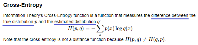
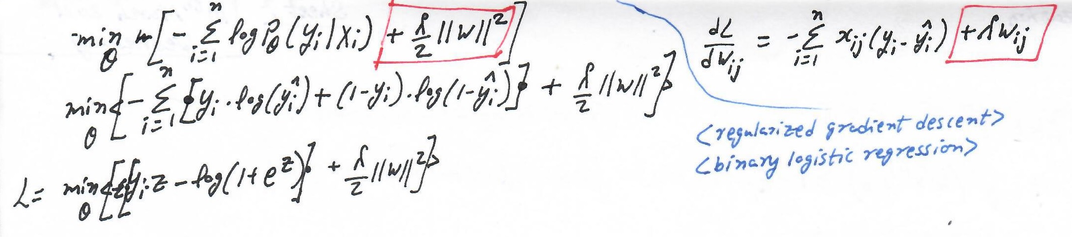
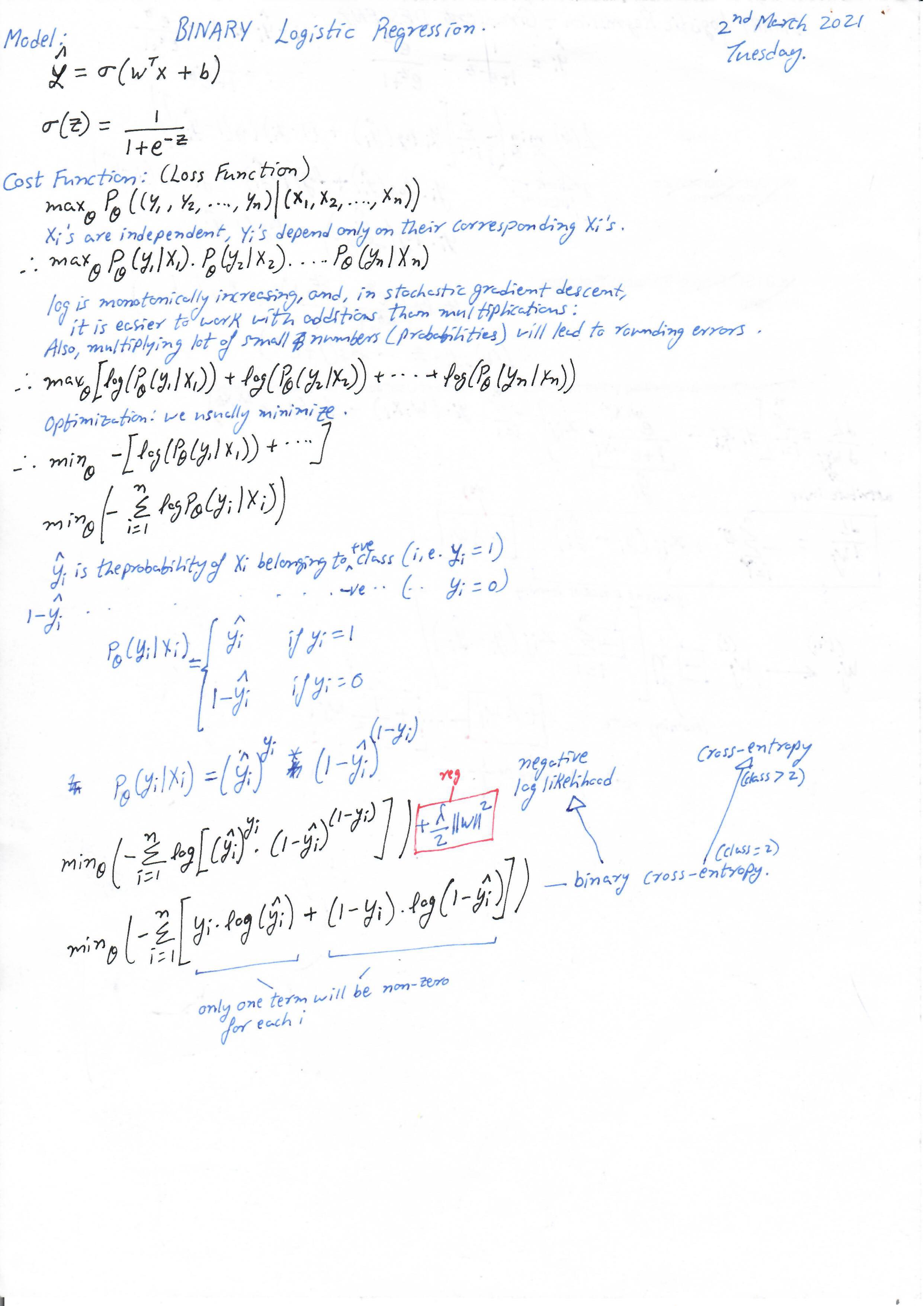
If we look at the equation below, the term ‘Y ln P(Y)’ is the cross entropy between the true probability Y (=1) and the predicted probability. Since when Y=1, we have (1-Y) = 0, and when Y=0, we have (1-Y) = 1, only one term per data point is non-zero. So, conditional data log-likelihood is basically a sum of cross entropies. The lower the cross entropy, the better the prediction. Hence, this function is a cost (loss) function.
#conditional data log-likelihood ln(P(Y|X,W))
def cond_data_log_likelihood(X_m, Y, w):
    likelihood = 0.0
    for i in range(len(X_m)):
        likelihood += (Y[i]*log(prob_y1_x(w, X_m[i])) + (1 - Y[i])*log(prob_y0_x(w, X_m[i])) )
    return (likelihood)
Gradient along attribute 'i'
#gradient along the attribute 'j'
def gradient(X_m, Y, W, j):
    grad = 0.0
    #iterate over all data-points
    for i in range(len(X_m)):
        grad += X_m[i][j]*(Y[i] - prob_y1_x(W, X_m[i]))
    return grad
Gradients along attributes
#gradient along each attribute
def gradients(X_m, Y, W):
    #gradient along each attribute
    grads = np.zeros(len(W), dtype=float)
    for j in range(len(W)):
        grads[j] = gradient(X_m, Y, W, j)

    return grads
Apply gradients on coefficients
def apply_gradient(W, grads, learning_rate):
    return (W + (learning_rate * grads))
Training Algorithm
def train(X_m, Y, W, learning_rate):
    #learn
    prev_max = cond_data_log_likelihood(X_m, Y, W)
    grads = gradients(X_m, Y, W)
    W = apply_gradient(W, grads, learning_rate)
    new_max = cond_data_log_likelihood(X_m, Y, W)
    #summary print
    i_print = 0
    while(abs(prev_max - new_max) > convergence_cost_diff):
        if(i_print % 500) == 0:
            print('Cost:', prev_max)
        prev_max = new_max
        grads = gradients(X_m, Y, W)
        W = apply_gradient(W, grads, learning_rate)
        new_max = cond_data_log_likelihood(X_m, Y, W)
        i_print += 1

    return W
Learn
#weights
W = np.zeros((n_features), dtype=float)
W = train(X_m, Y, W, learning_rate)
Cost: -69.31471805599459
Cost: -49.707947324850565
Cost: -40.87854558929088
Cost: -35.85466773616585
Cost: -32.65388264792396
Cost: -30.444903169173813
Cost: -28.830852125987995
Cost: -27.600808997259257
Cost: -26.63289105803656
Cost: -25.8518897927959
Cost: -25.20890607913062
Cost: -24.670769018536692
Cost: -24.21417569334356
Cost: -23.822268801602643
Cost: -23.482546876964133
Cost: -23.18553887871831
weights (coefficients)
print('The learnt weights (coefficients) are:', W)
The learnt weights (coefficients) are: [-14.97508012 1.16796148 1.35110071]
Prediction
Generate Data
Gaussian clusters in 2D numpy arrays
X_m, Y = generate_X_m_and_Y(M, K, n_features, loc_scale) #generate test data points
Predict
Y_pred = [prob_y1_x(W, X) for X in X_m]
Y_pred_class = [0 if y < 0.5 else 1 for y in Y_pred] #decision based on predicted margin
Predicted X_m, Y in DataFrame
df = create_df_from_array(X_m, Y, n_features, cols) #create test dataframe
df['Y_pred_margin'] = Y_pred #append the prediction margin column
df['Y_pred_class'] = Y_pred_class #append the class
df.sample(n = 10)
| X0 | X1 | X2 | Y | Y_pred_margin | Y_pred_class | |
|---|---|---|---|---|---|---|
| 37 | 1.0 | 5.234051 | 5.226969 | 0 | 0.141882 | 0 |
| 47 | 1.0 | 4.146087 | 6.144546 | 0 | 0.138154 | 0 |
| 22 | 1.0 | 6.182099 | 3.720378 | 0 | 0.061340 | 0 |
| 27 | 1.0 | 5.694109 | 5.687429 | 0 | 0.345181 | 0 |
| 43 | 1.0 | 5.386995 | 2.323051 | 0 | 0.003893 | 0 |
| 38 | 1.0 | 5.202220 | 5.670654 | 0 | 0.224878 | 0 |
| 99 | 1.0 | 7.099939 | 7.113818 | 1 | 0.949255 | 1 |
| 79 | 1.0 | 7.165353 | 6.450322 | 1 | 0.891757 | 1 |
| 29 | 1.0 | 4.034987 | 5.389770 | 0 | 0.048326 | 0 |
| 66 | 1.0 | 6.995258 | 6.390637 | 1 | 0.861703 | 1 |
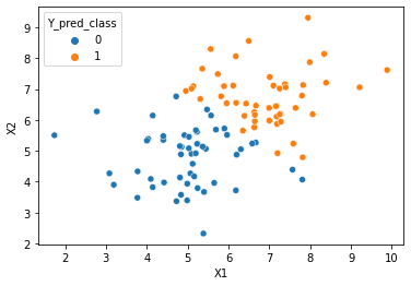
#scatter plot of data points
#class column Y is passed in as hue
sns.scatterplot(x=cols[1], y=cols[2], hue='Y_pred_class', data=df)
<AxesSubplot:xlabel='X1', ylabel='X2'>
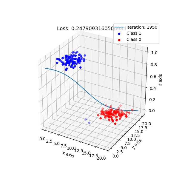
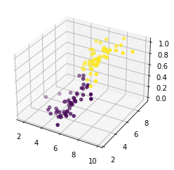
Y_pred_np = np.array(Y_pred)
fig = plt.figure()
ax = plt.axes(projection='3d')
ax.scatter3D(X_m[:, 1], X_m[:, 2], Y_pred, c = (Y_pred_np>0.5))
plt.show()
Prediction Accuracy
Y_pred_corr = (Y==Y_pred_class)
num_corr = len(Y_pred_corr[Y_pred_corr == True])
print('Accuracy:', (num_corr/M)*100, '%')
Accuracy: 88.0 %
Sidebar - Binomial Logistic Regression
P(Y|X) directly?
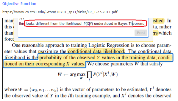
Actually, the term likelihood can be used for P(X|Y) as well as P(Y|X). It can be used for any distribution. In Naive Bayes, we estimate params (mu/sigma, or frequencies) for distribution P(X|Y). But, in Logistic Regression, we estimate W (the weight vector W in W.X) to maximize likelihood of the distribution P(Y|X) - this is what we call as estimating P(Y\|X) directly.
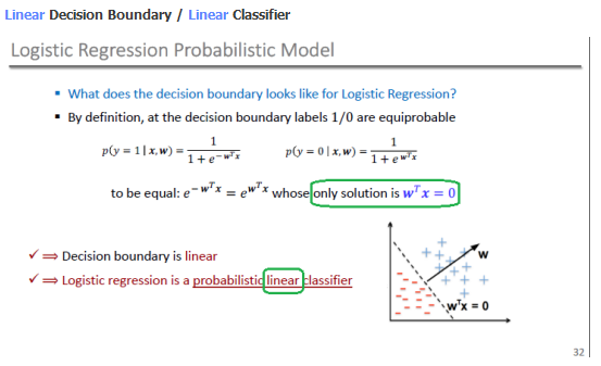
Linear Boundary
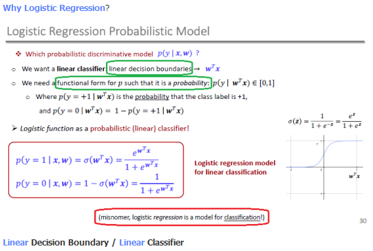
Why Logistic Regression?
Model and Cost Function
Derivatives for Gradient Descent
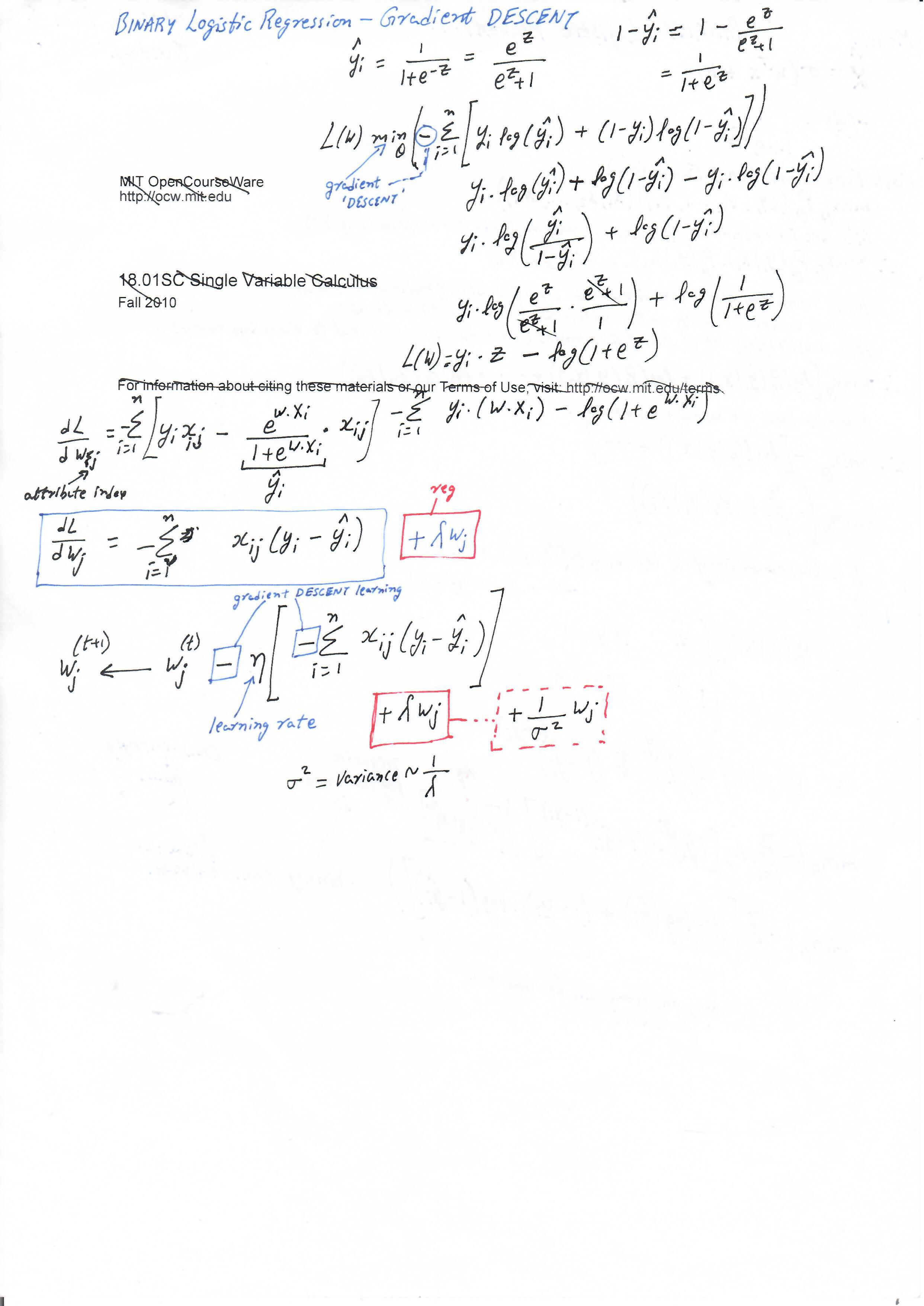
Regularized Logistic Regression