Visualizations Playground
For 3D 3-D 3-dimensional graphs using matplotlib, refer: https://jakevdp.github.io/PythonDataScienceHandbook/04.12-three-dimensional-plotting.html
Imports, and Data Fetch
imports
%matplotlib inline#imports
import matplotlib
import matplotlib.pyplot as plt
%matplotlib inline
#sns - Samuel Norman “Sam” Seaborn - on the television serial drama The West Wing
import seaborn as sns
import pandas as pd
import numpy as np
read configuration file
#configuration
from read_config import Config
config = Config ()
data
tips
config.set_dataset_id ("tips")
df_tips = config.get_train_df ()
df_tips.head (2)
| total_bill | tip | sex | smoker | day | time | size | |
|---|---|---|---|---|---|---|---|
| 0 | 16.99 | 1.01 | Female | No | Sun | Dinner | 2 |
| 1 | 10.34 | 1.66 | Male | No | Sun | Dinner | 3 |
iris
config.set_dataset_id ("iris")
df_iris = config.get_train_df ()
df_iris.head (2)
| Id | SepalLengthCm | SepalWidthCm | PetalLengthCm | PetalWidthCm | Species | |
|---|---|---|---|---|---|---|
| 0 | 1 | 5.1 | 3.5 | 1.4 | 0.2 | Iris-setosa |
| 1 | 2 | 4.9 | 3.0 | 1.4 | 0.2 | Iris-setosa |
titanic
config.set_dataset_id ("titanic")
df_titanic = config.get_train_df ()
df_titanic.head (2)
| PassengerId | Survived | Pclass | Name | Sex | Age | SibSp | Parch | Ticket | Fare | Cabin | Embarked | |
|---|---|---|---|---|---|---|---|---|---|---|---|---|
| 0 | 1 | 0 | 3 | Braund, Mr. Owen Harris | male | 22.0 | 1 | 0 | A/5 21171 | 7.2500 | NaN | S |
| 1 | 2 | 1 | 1 | Cumings, Mrs. John Bradley (Florence Briggs Th... | female | 38.0 | 1 | 0 | PC 17599 | 71.2833 | C85 | C |
matplotlib.pyplot TODO
https://jakevdp.github.io/PythonDataScienceHandbook/06.00-figure-code.html#Digits-Pixel-Components
- axis
- annotate
- set
- scatter
- axis
- imshow
- cmap
- interpolation
- clim
- plt
- subplots
- subplot_kw
- xticks
- yticks
- gripspec_kw
- hspace
- wspace
- subplot_kw
- figure
- GridSpec
- xlabel
- ylabel
- colorbar
- subplots
- figure
- add_subplot
- gridspec
- https://matplotlib.org/tutorials/intermediate/gridspec.html
Dataframe.plot ()
Plot Stacked Bar Charts, for the ‘Survived’ and ‘Not Survived’ filters, for various fields.
Prepare a dataframe - using list of series
Define a function that creates two series from the same field. The series are one each for ‘Survived’, and ‘Didn’t Survive’, and we use the ‘Survived’ field as a filter to separate the two series.
filter = df [col_filter] == value
df [filter][col].value_counts ()
def get_field_subtotals (field_name):
    f_survived = df_titanic ['Survived'] == 1
    s_survived = df_titanic [f_survived][field_name]\
    .value_counts ()

    f_not_survived = df_titanic ['Survived'] != 1
    s_not_survived = df_titanic [f_not_survived][field_name]\
    .value_counts ()

    return [s_survived, s_not_survived]
example usage
get_field_subtotals ('Sex')
[female    233
 male      109
 Name: Sex, dtype: int64, male      468
 female     81
 Name: Sex, dtype: int64]
Below, this is how a data frame created using get_field_subtotals () looks like. Since the two series are returned in a list, each series forms a row. The index of the series forms the column names. The name of each series is the field it was created from (‘Sex’). These names form the index of the data frame.
pd.DataFrame (get_field_subtotals ('Sex'))
| female | male | |
|---|---|---|
| Sex | 233 | 109 |
| Sex | 81 | 468 |
pd.DataFrame (get_field_subtotals ('Sex')).index
Index(['Sex', 'Sex'], dtype='object')
We should change the index values to something meaningful, like, the filter we used to segregate the rows into two series.
pd.DataFrame (get_field_subtotals ('Sex'),\
              index = ['Survived', 'Didn''t Survive'])
| female | male | |
|---|---|---|
| Survived | 233 | 109 |
| Didnt Survive | 81 | 468 |
Prepare a data frame - using df.groupby ().size ().unstack ()
df = df_titanic.groupby (['Survived', 'Sex']).size ().unstack ()
df
| Sex | female | male |
|---|---|---|
| Survived | ||
| 0 | 81 | 468 |
| 1 | 233 | 109 |
How to plot the data frames
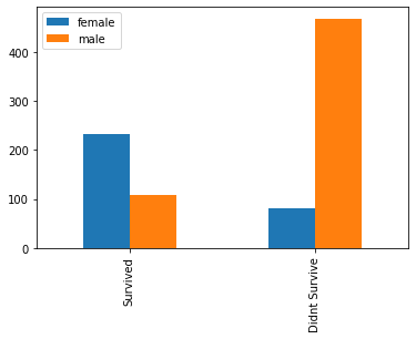
Unstacked Bar Chartusing data frame created from list of series
df.plot(kind = ‘bar’)
pd.DataFrame (get_field_subtotals ('Sex'),\
              index = ['Survived', 'Didn''t Survive'])\
.plot (kind = 'bar')
plt.show ()
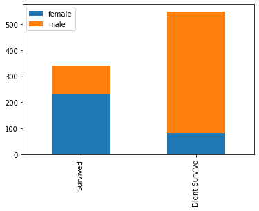
using data frame created from list of series
df.plot (kind = ‘bar’, stacked = 'True')
pd.DataFrame (get_field_subtotals ('Sex'), \
              index = ['Survived', 'Didn''t Survive']) \
.plot (kind = 'bar', stacked = 'True')
plt.show ()
using data frame created from groupby.size.unstack
groupby on two fields,
- the first field in the groupby clause is plotted on the X-axis
this is the index of the dataframe returned from unstack ()
- the second field in the groupby clause forms the Y-axis
this is the unstacked feature that forms columns in the dataframe returned from unstack ()
df_titanic.groupby (['Survived', 'Sex'])\
.size ().unstack ()\
.plot (kind = 'bar', stacked = True)
plt.show ()

Define a helper function that plots the data frame.
def plot_stacked_bar_chart (df, l_fields):
    df.groupby (l_fields).size ().unstack ()\
    .plot (kind = 'bar', stacked = True)
    plt.show ()
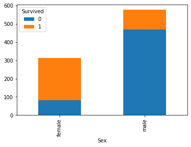
example usage, plot ‘Sex’ stacked bar
plot_stacked_bar_chart (df_titanic, ['Survived', 'Sex'])
example usage, plot ‘Pclass’ stacked bar
plot_stacked_bar_chart (df_titanic, ['Survived', 'Pclass'])
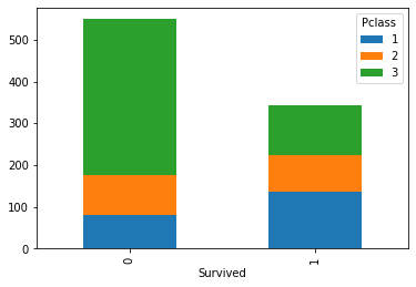
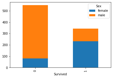
using data frame created from groupby.size.unstack (col_name)
We mention Survived as the feature to be unstacked.
df_titanic.groupby (['Survived', 'Sex'])\
.size ().unstack ('Survived')\
.plot (kind = 'bar', stacked = True)
plt.show ()
Seaborn
Seaborn is built on matplotlib
As for Seaborn, you have two types of functions: axes-level functions and figure-level functions. The ones that operate on the Axes level are, for example, regplot(), boxplot(), kdeplot(), …, while the functions that operate on the Figure level are lmplot(), factorplot(), jointplot() and a couple others.
The way you can tell whether a function is “figure-level” or “axes-level” is that axes-level functions takes an ax= parameter. You can also distinguish the two classes by their output type: axes-level functions return the matplotlib axes, while figure-level functions return the FacetGrid.
Axes-level functions
Axes-levelfunctions
- violinplot ()
- swarmplot ()
- scatterplot ()
- boxplot ()
- kdeplot ()
- regplot ()
returns matplotlib.axes._subplots.AxesSubplot
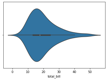
violinplot - tips
sns.violinplot (x = colname, data = df)
sns.violinplot (x = 'total_bill', data = df_tips)
plt.show ()
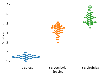
swarmplot - iris
sns.swarmplot (x = dim_x, y = dim_y, data = df)
sns.swarmplot (x = 'Species', y = 'PetalLengthCm', data = df_iris)
plt.show ()
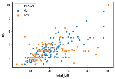
scatterplot - tips
sns.scatterplot (dim_x, dim_y, data = )
*scatterplot is suitable for both continuous and discrete variables.
sns.scatterplot ("total_bill", "tip", "smoker", data = df_tips)
plt.show ()
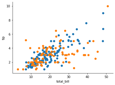
scatterplot plot using a FacetGrid
fg = sns.FacetGrid (df_tips, hue = "smoker", height = 4, aspect = 1.33)
fg.map (plt.scatter, "total_bill", "tip")
plt.show ()
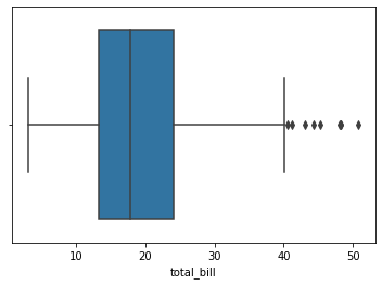
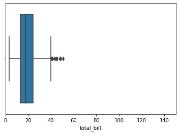
boxplot - tips
sns.boxplot (x = dim_x, data = df)
sns.boxplot (x = "total_bill", data = df_tips)
plt.show ()
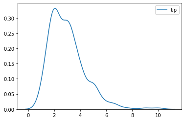
kdeplot - titanic
sns.kdeplot (df[col])
sns.kdeplot (df_tips["tip"])
plt.show ()
heatmap - titanic
sns.heatmap (df.corr ())
df_temp = df_titanic.drop (['PassengerId', 'Name', \
                  'Cabin', 'SibSp', 'Parch'], axis = 1)
sns.heatmap (df_temp.corr ())
plt.show ()
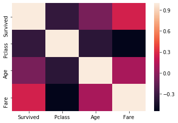
Figure-level functions
Figure-levelfunctions
- lmplot () - Linear [regression] Model
- catplot () - was known as factorplot ()
- jointplot () - illuminating the structure of a dataset
- pairplot () - illuminating the structure of a dataset
returns seaborn.axisgrid.FacetGrid
FacetGrid.axes returns the axes
These are optimized for exploratory analysis because they set up the matplotlib figure containing the plot(s) and make it easy to spread out the visualization across multiple axes. They also handle some tricky business like putting the legend outside the axes. To do these things, they use a seaborn FacetGrid.
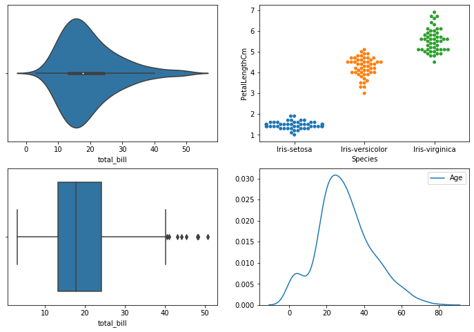
1. Figure-level and axes-level functions
Each different figure-level plot kind combines a particular “axes-level” function with the FacetGrid object. For example, the scatter plots are drawn using the scatterplot() function, and the bar plots are drawn using the barplot() function. These functions are called “axes-level” because they draw onto a single matplotlib axes and don’t otherwise affect the rest of the figure.
The upshot is that the figure-level function needs to control the figure it lives in, while axes-level functions can be combined into a more complex matplotlib figure with other axes that may or may not have seaborn plots on them:
fig, ax = plt.subplots (2, 2, figsize = (12, 8))
sns.violinplot (x = 'total_bill', data = df_tips, ax = ax[0][0])
sns.swarmplot (x = 'Species', y = 'PetalLengthCm', data = df_iris, ax = ax[0][1])
sns.boxplot (x = "total_bill", data = df_tips, ax = ax[1][0])
sns.kdeplot (df_titanic ["Age"], ax = ax[1][1])
plt.show ()
/opt/anaconda3/lib/python3.7/site-packages/statsmodels/nonparametric/kde.py:447: RuntimeWarning: invalid value encountered in greater
  X = X[np.logical_and(X > clip[0], X < clip[1])] # won't work for two columns.
/opt/anaconda3/lib/python3.7/site-packages/statsmodels/nonparametric/kde.py:447: RuntimeWarning: invalid value encountered in less
  X = X[np.logical_and(X > clip[0], X < clip[1])] # won't work for two columns.
Controlling the size of the figure-level functions works a little bit differently than it does for other matplotlib figures. Instead of setting the overall figure size, the figure-level functions are parameterized by the size of each facet. And instead of setting the height and width of each facet, you control the height and aspect ratio (ratio of width to height). This parameterization makes it easy to control the size of the graphic without thinking about exactly how many rows and columns it will have, although it can be a source of confusion.
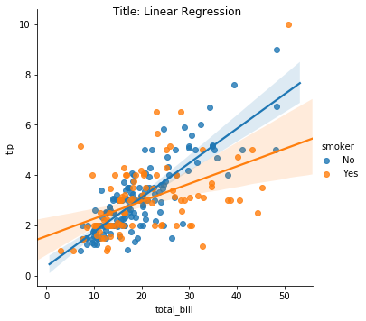
2. Statistical Estimation
lmplot
lmplot(x = , y = , data = )
FacetGrid.fig.suptitle ()
fgrid = sns.lmplot (x = "total_bill", y = "tip", hue = "smoker", \
                 data = df_tips)
# Add a title to the Figure
fig = fgrid.fig
fig.suptitle('Title: Linear Regression', fontsize=12)
plt.show ()
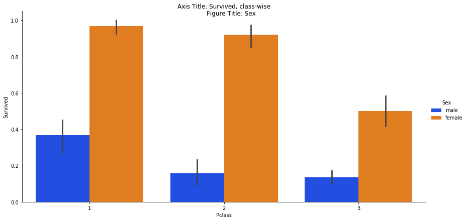
3. Specialized Categorical Plots
catplot
exposes a common dataset-oriented API that generalizes over different representations of the relationship between one numeric variable and one (or more) categorical variables.
sns.catplot (dim_x, dim_y, dim_z, data = df, kind = bar, palette = )
‘Survived’ is numerical
Controlling the size of the figure-level functions works a little bit differently than it does for other matplotlib figures. Instead of setting the overall figure size, the figure-level functions are parameterized by the size of each facet. And instead of setting the height and width of each facet, you control the height and aspect ratio (ratio of width to height). This parameterization makes it easy to control the size of the graphic without thinking about exactly how many rows and columns it will have, although it can be a source of confusion.
fgrid = sns.catplot (x = "Pclass", y = "Survived", hue = "Sex",\
             data = df_titanic, \
                kind = "bar", palette = "bright",\
             height = 6, aspect = 2)
ax = fgrid.ax
ax.set_title ('Axis Title: Survived, class-wise')
fig = fgrid.fig
fig.suptitle ('Figure Title: Sex')
plt.show ()
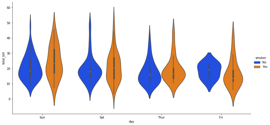
sns.catplot (dim_x, dim_y, dim_z, data = df, kind = violin, palette = )
‘total_bill’ is numerical
sns.catplot (x = "day", y = "total_bill", hue = "smoker",\
             data = df_tips, \
                kind = "violin", palette = "bright",\
             height = 6, aspect = 2)
plt.show ()
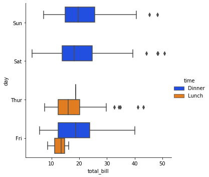
sns.catplot (dim_x, dim_y, dim_z, data = df, kind = box, palette = )
‘total_bill’ is numerical
sns.catplot (x = "total_bill", y = "day", hue = "time",\
             data = df_tips, \
                kind = "box", palette = "bright")
plt.show ()
4. Visualizing Dataset Structure
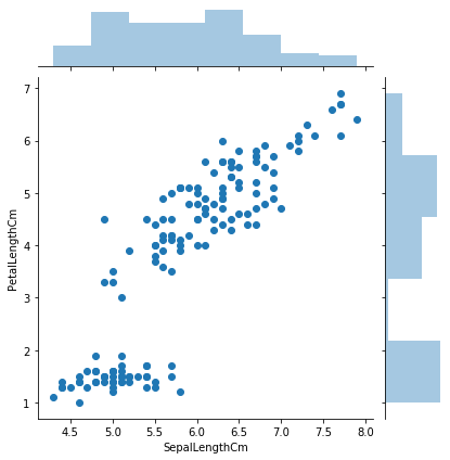
jointplot
sns.jointplot (x = , y = , data = )
focuses on a single relationship
sns.jointplot (x = "SepalLengthCm", y = "PetalLengthCm", data = df_iris)
plt.show ()
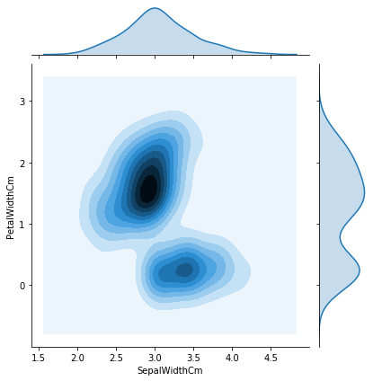
sns.jointplot (x = , y = , data = , kind = 'kde')
sns.jointplot (x = 'SepalWidthCm', y = 'PetalWidthCm', data = df_iris,\
               kind = 'kde')
plt.show ()
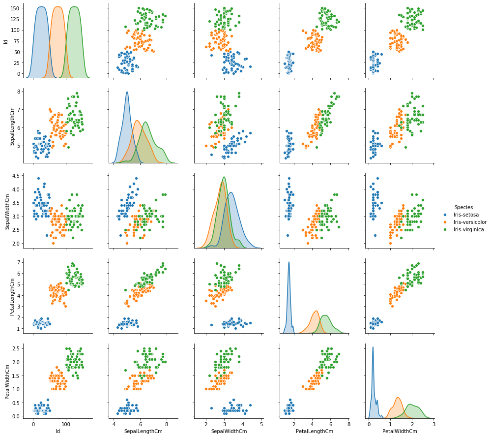
pairplot - iris
sns.pairplot (data = , hue = )
This plot takes a broader view, showing all pairwise relationships and the marginal distributions, optionally conditioned on a categorical variable
sns.pairplot (data = df_iris, hue = "Species")
plt.show ()
#returns matplotlib.axes._subplots.AxesSubplot
fig, ax = plt.subplots ()
ax.set (xlim = (0, 150))
ax = sns.boxplot (x = "total_bill", data = df_tips, ax = ax)
#ax.set (xlim = (0, 100))
plt.show ()
FacetGrid
A FacetGrid can be drawn with up to three dimensions − row, col, and hue. The first two have obvious correspondence with the resulting array of axes; think of the hue variable as a third dimension along a depth axis, where different levels are plotted with different colors.
The variables should be categorical and the data at each level of the variable will be used for a facet along that axis.
Warning: When using seaborn functions that infer semantic mappings from a dataset, care must be taken to synchronize those mappings across facets. In most cases, it will be better to use a figure-level function (e.g. relplot() or catplot()) than to use FacetGrid directly.
facet = sns.FacetGrid (df, row = , col = , hue = )
facet.map (plt.type, dim_x, [dim_y])
facet = sns.FacetGrid (df, col = )
facet.map (plt.hist, dim_x)
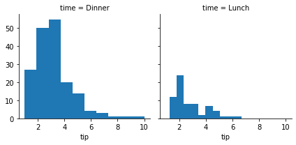
histogram is suitable for continuous variables. For discrete variables, we can use bar chart.
Tips
facet = sns.FacetGrid (df_tips, col = "time")
facet.map (plt.hist, "tip")
plt.show ()
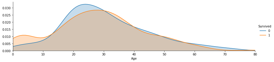
Plot a Probability Density Function of ‘Age’, from the Survived and Not Survived groups
facet = sns.FacetGrid (df, hue =)
facet.map (sns.kdeplot, dim_x)
KDE Plot described as Kernel Density Estimate is used for visualizing the Probability Density of a continuous variable. y-axis
variable to be plotted - x-axis
Titanic
facet = sns.FacetGrid (df_titanic, hue = 'Survived', aspect = 4)
facet.map (sns.kdeplot, 'Age', shade = True)
facet.set (xlim = (0, df_titanic ['Age'].max ()))
facet.add_legend ()
plt.show ()
facet = sns.FacetGrid (df, col = , hue =)
facet.map (plt.scatter, dim_x, dim_y)
Tips
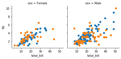
facet = sns.FacetGrid (df_tips, col = "sex", hue = "smoker")
facet.map (plt.scatter, "total_bill", "tip")
plt.show ()
facet = sns.FacetGrid (df, row =, col =, hue =)
facet.map (plt.scatter, dim_x, dim_y)
Tips
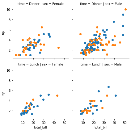
facet = sns.FacetGrid (df_tips, row = "time",\
                       col = "sex", hue = "smoker")
facet.map (plt.scatter, "total_bill", "tip")
plt.show ()
some customizations
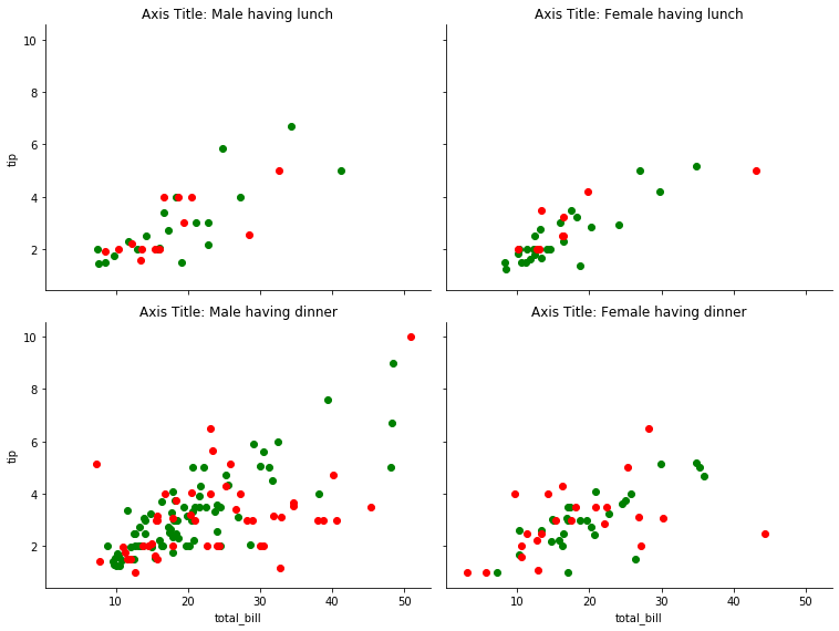
pal = {'Yes': 'red', 'No': 'green'}
fgrid = sns.FacetGrid (df_tips, row = "time", col = "sex", \
                    col_order = ['Male', 'Female'], \
                    row_order = ['Lunch', 'Dinner'], \
                    hue = "smoker", \
                    height = 4, aspect = 1.33, \
                   palette = pal)
fgrid.map (plt.scatter, "total_bill", "tip")

#titles
ax = fgrid.axes
ax[0][0].set_title ('Axis Title: Male having lunch')
ax[0][1].set_title ('Axis Title: Female having lunch')
ax[1][0].set_title ('Axis Title: Male having dinner')
ax[1][1].set_title ('Axis Title: Female having dinner')
fig = fgrid.fig
#fig.suptitle ('Figure Title: Total Bill and Tips across dimensions')

plt.show ()
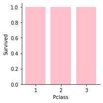
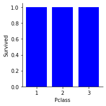
problems with hue
FacetGrid can also represent levels of a third variable with the hue parameter, which plots different subsets of data in different colors. This uses color to resolve elements on a third dimension, but only draws subsets on top of each other and will not tailor the hue parameter for the specific visualization the way that axes-level functions that accept hue will.
Tips
pal = {'male': 'blue', 'female': 'pink'}
fg = sns.FacetGrid (df_titanic, hue = "Sex", \
                    hue_order = ['female', 'male'], \
                   palette = pal)
fg.map (plt.bar, 'Pclass', 'Survived')
plt.show ()
pal = {'male': 'blue', 'female': 'pink'}
fg = sns.FacetGrid (df_titanic, hue = "Sex", \
                    hue_order = ['male', 'female'], \
                   palette = pal)
fg.map (plt.bar, 'Pclass', 'Survived')
plt.show ()