SciPy Playground
NumPy provides some functions for Linear Algebra, Fourier Transforms and Random Number Generation, but not with the generality of the equivalent functions in SciPy.
Imports
#multi-dimensional array
import numpy as np
from numpy import vstack #vertical stacking of arrays

#random sampling from distributions
from numpy.random import rand, randn, normal, standard_normal

#data normalization
from scipy.cluster.vq import whiten

#clustering
from scipy.cluster.vq import kmeans #clustering algorithm
#optimization
from scipy import optimize

#classification
#vector quantization - quantizing (labeling) vectors by
# comparing them with centroids
from scipy.cluster.vq import vq

#put ndarrays into a dataframe for plotting
import pandas as pd

#visualizations
import matplotlib
import matplotlib.pyplot as plt
%matplotlib inline
#sns - Samuel Norman “Sam” Seaborn -
# on the television serial drama The West Wing
import seaborn as sns

#representing sparse martices
from scipy.sparse import csr_matrix # 'compressed sparse row' matrix
from scipy.sparse import dok_matrix # 'dictionary of keys' matrix

#integration
from scipy.integrate import quad, dblquad

#interpolation
from scipy import interpolate
from scipy.interpolate import interp1d

#generated data
import generate_data as gd
scipy.interpolate
https://www.tutorialspoint.com/scipy/scipy_interpolate.htm
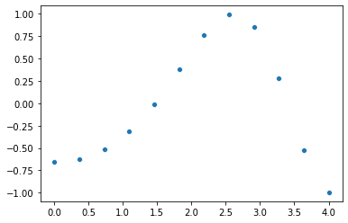
plot a function of x
cos ( (x_square/3) + 4)
#a set of equidistant points within an interval
x = np.linspace (0, 4, 12)

#a function of x
#cos ( (x_square/3) + 4)
y = np.cos (((x**2)/3) + 4)

#plot
sns.scatterplot (x, y)
plt.show ()
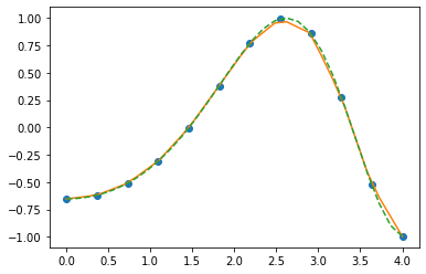
using interpolation, fit a function to the points
f1d_lin = interp1d (x, y, kind = 'linear')
f1d_cub = interp1d (x, y, kind = 'cubic')
x_val = 2
print ('1D Linear interpolation estimate for x =', x_val,\
       ':', f1d_lin (x_val))
print ('1D Cubic interpolation estimate for x =', x_val,\
       ':', f1d_cub (x_val))
1D Linear interpolation estimate for x = 2 : 0.5734566736497806
1D Cubic interpolation estimate for x = 2 : 0.5820766474144136
Note
- if we reduce the number of points on which interpolation was performed, we see the effect of cubic interpolation error due to overfitting
- for x = np.linspace (0, 4, 6)
- 1D Linear interpolation estimate for x = 2 : 0.5376240708619846
- 1D Cubic interpolation estimate for x = 2 : 0.6162970299094371
plot the interpolation output
x_vals = np.linspace (0, 4, 30) #input x to the learnt functions
y_vals_lin = f1d_lin (x_vals) #output y from the learnt linear function
y_vals_cub = f1d_cub (x_vals) #output y from the learnt cubic function
plt.plot (x, y, 'o',\
         x_vals, y_vals_lin, '-',\
         x_vals, y_vals_cub, '--')
plt.show ()
scipy.integrate
http://kitchingroup.cheme.cmu.edu/blog/2013/02/02/Integrating-functions-in-python/
integrands
#x_square
def integrand_single (x):
    return x**2

# $x$y y.sin(x) + x.cos(y)
#inner-most integral variable should be the first parameter
def integrand_double (y, x):
    return y * np.sin (x) + x * np.cos (y)
evaluate
# integrate x_square
# x = 0..1
ans, err = quad (integrand_single, 0, 1)
print ('\nintegrate x_square from x = 0..1:', ans, err)

# $x$y y.sin(x) + x.cos(y)
# π<=x<=2π
# 0<=y<=π
#We have to provide callable functions for the range of the y-variable.
#Here they are constants, so we create lambda functions
# that return the constants.
ans, err = dblquad (integrand_double, np.pi, 2 * np.pi,\
                   lambda x: 0, lambda x: np.pi)
print ('\nintegrate $x$y y.sin(x) + x.cos(y) from\n π<=x<=2π and 0<=y<=π:',\
       ans, err)
integrate x_square from x = 0..1: 0.33333333333333337 3.700743415417189e-15

integrate $x$y y.sin(x) + x.cos(y) from
 π<=x<=2π and 0<=y<=π: -9.869604401089358 1.4359309630105241e-13
scipy.optimize
https://towardsdatascience.com/optimization-with-scipy-and-application-ideas-to-machine-learning-81d39c7938b8
Using SciPy gives you deep insight into the actual working of the algorithm as you have to construct the loss metric yourself and not depend on some ready-made, out-of-the-box function.
Single-Variate Objective Functions
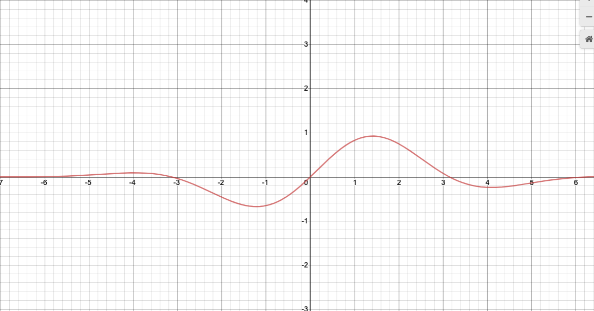
Plot and Definition
#parabola
def parabola (x):
    return x**2

#exotic - sin (x) * exp [-0.1 (x - 0.6)^2]
def sinx_exp  (x):
    return np.sin (x) * np.exp (-0.1 * ((x - 0.6) ** 2))

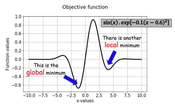
Optimization
1. without constraints, without bounds
optimize.minimize_scalar (objfn)
result = optimize.minimize_scalar (parabola)
print ('minimum of parabola:\n', result)
result = optimize.minimize_scalar (sinx_exp)
print ('\nminimum of sinx_exp:\n', result)
minimum of parabola:
      fun: 0.0
    nfev: 8
     nit: 4
 success: True
       x: 0.0

minimum of sinx_exp:
      fun: -0.6743051024666711
    nfev: 15
     nit: 10
 success: True
       x: -1.2214484245210282
2. with bounds (constraints)
- For sinx-exp, mention bounds on x so as to favor local minimum
optimize.minimize_scalar (objfn, bounds = , method = ‘Bounded’)
result = optimize.minimize_scalar (sinx_exp, bounds = (0, 10), \
                                  method = 'Bounded')
print ('\nminimum of sinx_exp:\n', result)
minimum of sinx_exp:
      fun: -0.24037563941326692
 message: 'Solution found.'
    nfev: 12
  status: 0
 success: True
       x: 4.101466164987216
3. with other functional constraints
sinx_exp constraints

def constraint1 (x):
    return (0.5 - np.log10 (x**2 + 2))
def constraint2 (x):
    return (np.log10 (x**2 + 2) - 1.5)
def constraint3 (x):
    return (np.sin (x) + (0.3 * (x**2)) - 1)

print ('Graphically, constraints met at x = -2.3757.')
print ('Passing x = -2.3757 in constraint functions:\n')
print ('Constraint #1 < 0:', constraint1 (-2.3757))
print ('Constraint #2 < 0:', constraint2 (-2.3757))
print ('Constraint #3 = 0 (almost equal to 0):', constraint3 (-2.3757))

#prepare a dictionary for each constraint
con1 = {'type': 'ineq', 'fun': constraint1} #Inequality
con2 = {'type': 'ineq', 'fun': constraint2} #Inequality
con3 = {'type': 'eq', 'fun': constraint3} #Equality

#prepare a tuple of constraints
cons = (con1, con2, con3)

print (type(con1))
print (type(con2))
print (type(con3))
#print (type(con))
#for ic, con in cons:
    #print (ic, con)
Graphically, constraints met at x = -2.3757.
Passing x = -2.3757 in constraint functions:

Constraint #1 < 0: -0.38331786545918767
Constraint #2 < 0: -0.6166821345408123
Constraint #3 = 0 (almost equal to 0): 4.4798883980234905e-06
<class 'dict'>
<class 'dict'>
<class 'dict'>
optimize.minimize (objfn, bounds = , method = ‘Bounded’)
SciPy allows handling arbitrary constraints through the more generalized method optimize.minimize.
Note:
- not all methods in the minimize function support constraint and bounds).
- Here we chose SLSQP method which stands for sequential least-square quadratic programming
- to use minimize we need to pass on an initial guess in the form of x0 argument
This code fails to optimize
result = optimize.minimize (sinx_exp, x0 = 0, method = 'SLSQP', \
                                  constraints = cons,\
                           options = {'maxiter': 100})
print ('\nminimum of sinx_exp:\n', result)
print ('\nNote the ERROR!!!: success: False')
minimum of sinx_exp:
      fun: array([0.76316959])
     jac: array([0.59193639])
 message: 'Iteration limit reached'
    nfev: 392
     nit: 100
    njev: 100
  status: 9
 success: False
       x: array([0.8773752])

Note the ERROR!!!: success: False
provide a suitable initial guess of x0 = -2
result = optimize.minimize (sinx_exp, x0 = -2, method = 'SLSQP', \
                                  constraints = cons,\
                           options = {'maxiter': 100})
print ('\nminimum of sinx_exp:\n', result)
print ('\nNote the SUCCESS!!!: success: True')
minimum of sinx_exp:
      fun: array([-0.28594945])
     jac: array([-0.46750661])
 message: 'Positive directional derivative for linesearch'
    nfev: 12
     nit: 76
    njev: 6
  status: 8
 success: False
       x: array([-2.37569791])

Note the SUCCESS!!!: success: True
reduce the number of iterations from 100 down to 3
This code fails with iteration limit, but succeeds to get good enough optimization
result = optimize.minimize (sinx_exp, x0 = -2, method = 'SLSQP', \
                                  constraints = cons,\
                           options = {'maxiter': 3})
print ('\nminimum of sinx_exp:\n', result)
print ('\nNote the FAILURE!!!: success: False')
print ('But, the resultant x is close to the success case.')
minimum of sinx_exp:
      fun: array([-0.2854205])
     jac: array([-0.46737936])
 message: 'Iteration limit reached'
    nfev: 6
     nit: 3
    njev: 3
  status: 9
 success: False
       x: array([-2.37682949])

Note the FAILURE!!!: success: False
But, the resultant x is close to the success case.
Multi-variate Objective Functions
Plot and Definition
Gaussian Mixture
- gauss 1: mean = -1, sd = 2.1
- gauss 2: mean = 0.3, sd = 0.8
- gauss 1: mean = 2.1, sd = 1.7


#expects a vetor x
def gaussian_mixture (x):

    gausses = []
    for i in range (len(x)):
        gauss = np.exp (-((x[i]-means[i])**2)/(stds[i]**2))
        gausses.append (gauss)

    #objective function is formulated as a function to be minimized
    #maximizing the gaussians is minimizing their negative
    return -1 * sum(gausses)
Optimization
Unbounded Inputs - optimize.minimize (objfn, method = ‘SLSQP’)
- gauss 1: mean = -1, sd = 2.1
- gauss 2: mean = 0.3, sd = 0.8
- gauss 1: mean = 2.1, sd = 1.7
Note:
- we get back a vector instead of a scalar
- the code below returns an array of means of the respective distributuions.
means = [-1, 0.3, 2.1]
stds = [2.1, 0.8, 1.7]
initial_guess = np.zeros ((3))
result = optimize.minimize (gaussian_mixture, x0 = initial_guess,\
                           method = 'SLSQP',\
                           options = {'maxiter': 100})
print (result)
print ('\nObserve that x is the means of the respective distributuions')
     fun: -2.9999996182234456
     jac: array([-8.10027122e-05, -2.40176916e-04,  7.11083412e-04])
 message: 'Optimization terminated successfully'
    nfev: 34
     nit: 8
    njev: 8
  status: 0
 success: True
       x: array([-1.00017856,  0.29992314,  2.1010275 ])

Observe that x is the means of the respective distributuions
Bounded Inputs - optimize.minimize (objfn, bounds = , method = ‘SLSQP’)
If the sub-process settings can occupy only a certain range of values (some must be positive, some must be negative, etc.) then the solution will be slightly different — it may not be the global optimum.
means = [-1, 0.3, 2.1]
stds = [2.1, 0.8, 1.7]
initial_guess = np.zeros ((3))

x1_bound = (-2,2)
x2_bound = (0,5)
x3_bound = (-3,0)
bounds = (x1_bound, x2_bound, x3_bound)

result = optimize.minimize (gaussian_mixture, x0 = initial_guess,\
                           method = 'SLSQP',\
                           options = {'maxiter': 100},\
                           bounds = bounds)
print (result)
print ('\nObserve that x1 and x2 are still the means, \
while x3 has reduced to almost 0 due to the constraint.')
     fun: -2.2174140557543054
     jac: array([-2.89082527e-06,  3.59982252e-04, -3.15965086e-01])
 message: 'Optimization terminated successfully'
    nfev: 25
     nit: 6
    njev: 6
  status: 0
 success: True
       x: array([-1.00000636,  0.30011519,  0.        ])

Observe that x1 and x2 are still the means, while x3 has reduced to almost 0 due to the constraint.
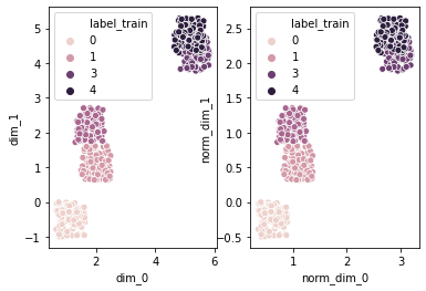
scipy.cluster
cluster settings
num_points = 100
num_dim = 2
num_clusters = 5
cluster_distance = 1
normalize = True
plot the data
#generate cluster data
df = gd.generate_cluster_data (num_points, \
                              num_dim, num_clusters, cluster_distance, \
                  normalize)

#plot the prepared data and its normalized form
fig, ax = plt.subplots (1, 2)#, figsize = (8, 8))
#parameters are created from column names using *[list]
sns.scatterplot (*(list(df.columns [:num_dim])), 'label_train',\
                 data = df, ax = ax [0])
#from col# num_dim to col# 2*num_dim, say, from col 2 to col 4 (excluding)
sns.scatterplot (*(list(df.columns [num_dim:2*num_dim])), 'label_train',\
                 data = df, ax = ax [1])

plt.show ()
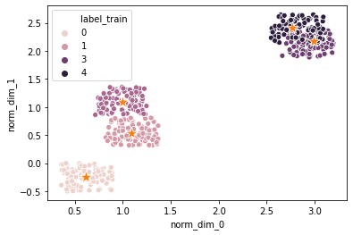
cluster the data
centroids = kmeans (data, n_clusters)
labels = vq (data, centroids)
# algorithm
data_norm = df [df.columns [num_dim:-1]].to_numpy ()
centroids, _ = kmeans (data_norm, num_clusters)
# classification
label_test, _ = vq (data_norm, centroids)

# plot

#plot the points
sns.scatterplot (*(list(df.columns [num_dim:2*num_dim])), 'label_train',\
                 data = df)

#plot the centroids
sns.scatterplot (centroids [:, 0], centroids [:, 1],\
                 marker = '*', s = 200)

plt.show ()
scipy.sparse, Sparse Matrix
Data Structures
Data
mat = np.array ([[1, 0, 0, 1, 0, 0], [0, 0, 2, 0, 0, 1],\
                    [0, 0, 0, 2, 0, 0]])
print ('2D array:\n', mat)
2D array:
 [[1 0 0 1 0 0]
 [0 0 2 0 0 1]
 [0 0 0 2 0 0]]
CSR (compressed sparse row) form
mat_csr = csr_matrix (mat)
print ('Compressed Sparse Row (CSR) form of 2D array:\n', mat_csr)
print ('CSR internals:\n', 'data: ', mat_csr.data,\
       'index pointer: ', mat_csr.indptr, 'indices: ', mat_csr.indices)
mat_dense_from_csr = mat_csr.todense ()
print ('Dense array got back from CSR form:\n', mat_dense_from_csr)
Compressed Sparse Row (CSR) form of 2D array:
   (0, 0)	1
  (0, 3)	1
  (1, 2)	2
  (1, 5)	1
  (2, 3)	2
CSR internals:
 data:  [1 1 2 1 2] index pointer:  [0 2 4 5] indices:  [0 3 2 5 3]
Dense array got back from CSR form:
 [[1 0 0 1 0 0]
 [0 0 2 0 0 1]
 [0 0 0 2 0 0]]
NOTE on CSR internals:
- indices [0, 3] are for row_0, [2, 5] are for row_1, [3] is for row_2
- indptr 0 points to start of row_0 indices, and 2 points to start of row_1 indices, etc
DoK (dictionary of keys) form
mat_dok = dok_matrix (mat)
print ('Dictionary of Keys (DoK) form of 2D array:\n',\
       list (mat_dok.items()))
mat_dense_from_dok = mat_dok.todense ()
print ('Dense array got back from DoK form:\n', mat_dense_from_dok)
Dictionary of Keys (DoK) form of 2D array:
 [((0, 0), 1), ((0, 3), 1), ((1, 2), 2), ((1, 5), 1), ((2, 3), 2)]
Dense array got back from DoK form:
 [[1 0 0 1 0 0]
 [0 0 2 0 0 1]
 [0 0 0 2 0 0]]
Calculate Sparsity
np.count_nonzero(ndarray) and np.ndarray.size
print ('Non-Zero count: ', np.count_nonzero (mat))
print ('Size: ', mat.size)
Non-Zero count:  5
Size:  18
density = nonzero_count / size sparcity = 1 - density
print ('Sparsity: ', 1 - (np.count_nonzero (mat) / mat.size))
Sparsity: 0.7222222222222222