NumPy or Numeric Python is a package for computation on homogenous n-dimensional arrays.

Uses:

perform operations on all the elements of two list directly.

A. Imports

#array handling
import numpy as np

#random sampling from distributions
from numpy.random import randn, normal, standard_normal

#plotting
from matplotlib import pyplot as plt
import seaborn as sns

B. Preliminaries

1. row vector, column vector, and matrix

All are of type numpy.ndarray

row_v = np.array ([0, 1, 2, 3, 4, 5, 6, 7, 8, 9]) # row vector (1-D)
# column vector (2-D)
col_v = np.array ([[0], [1], [2], [3], [4], [5], [6], [7], [8], [9]])
mat_2d = np.array ([[1, 'a'], [2, 'b'], [3, 'c']]) # 2-D matrix
mat_3d = np.array ([[[1, 'a'], [2, 'b'], [3, 'c']], \
                   [[4, 'd'], [5, 'e'], [6, 'f']], \
                   [[7, 'g'], [8, 'h'], [9, 'i']]]) # 3-D matrix

print ('row_v shape:', row_v.shape, '\n', row_v, '\n',\
       'element (1) of 1D array:', row_v[1], '\n')
print ('col_v shape:', col_v.shape, '\n', col_v, '\n',\
       'element (2,0) of 2D array:', col_v[2][0], '\n')
print ('mat_2d shape:', mat_2d.shape, '\n', mat_2d, '\n',\
       'element (2,1) of 2D array:', mat_2d[2][1], '\n')
print ('mat_3d shape:', mat_3d.shape, '\n', mat_3d, '\n',\
       'element (2,1,0) of 3D array:', mat_3d[2][1][0],\
       'element (2,2,1) of 3D array:', mat_3d[2][2][1],'\n')

row_v shape: (10,) 
 [0 1 2 3 4 5 6 7 8 9] 
 element (1) of 1D array: 1 

col_v shape: (10, 1) 
 [[0]
 [1]
 [2]
 [3]
 [4]
 [5]
 [6]
 [7]
 [8]
 [9]] 
 element (2,0) of 2D array: 2 

mat_2d shape: (3, 2) 
 [['1' 'a']
 ['2' 'b']
 ['3' 'c']] 
 element (2,1) of 2D array: c 

mat_3d shape: (3, 3, 2) 
 [[['1' 'a']
  ['2' 'b']
  ['3' 'c']]

 [['4' 'd']
  ['5' 'e']
  ['6' 'f']]

 [['7' 'g']
  ['8' 'h']
  ['9' 'i']]] 
 element (2,1,0) of 3D array: 8 element (2,2,1) of 3D array: i 

2. np.zeros, np.ones, and np.full

numerical arrays

np.zeros (shape, dtype = int/float)
np.ones (shape, dtype = int/float)

print (type (np.zeros ((1, 2), dtype = int))) #type
print ('integer 1D ndarray:\n',\
       np.zeros ((3), dtype = int), '\n') #integer 1D ndarray
print ('integer 2D ndarray:\n',\
       np.ones ((1, 2), dtype = int), '\n') #integer 2D ndarray
print ('float 2D ndarray:\n',\
       np.zeros ((1, 2), dtype = float), '\n') #float 2D ndarray
print ('float 3D ndarray:\n',\
       np.ones ((2, 3, 2), dtype = float), '\n') #float 3D ndarray

<class 'numpy.ndarray'>
integer 1D ndarray:
 [0 0 0] 

integer 2D ndarray:
 [[1 1]] 

float 2D ndarray:
 [[0. 0.]] 

float 3D ndarray:
 [[[1. 1.]
  [1. 1.]
  [1. 1.]]

 [[1. 1.]
  [1. 1.]
  [1. 1.]]] 

boolean arrays

np.zeros (shape, dtype = bool)

print ('boolean 2D ndarray:\n',\
       np.ones ((1, 2), dtype = bool), '\n')
print ('boolean 3D ndarray:\n',\
       np.ones ((2, 3, 2), dtype = bool), '\n')

boolean 2D ndarray:
 [[ True  True]] 

boolean 3D ndarray:
 [[[ True  True]
  [ True  True]
  [ True  True]]

 [[ True  True]
  [ True  True]
  [ True  True]]] 

any-type arrays

np.full (shape, value)

Deduce type from value

2D boolean array

np.full ((2,3), False)

array([[False, False, False],
       [False, False, False]])

2D integer array

np.full ((2,3), 7)

array([[7, 7, 7],
       [7, 7, 7]])

3. np.arange, and np.linspace

The essential difference between NumPy linspace and NumPy arange is that linspace enables you to control the precise end value, whereas arange gives you more direct control over the increments between values in the sequence.

np.arange (start = , stop = , step = )

only ‘stop’ is mandatory

print ('arange (10): stop at 10', np.arange (10))
print ('arange (-1, 10, 2): start at -1,\n \
stop at 10, step size = 2:', np.arange (-1, 10, 2))

arange (10): stop at 10 [0 1 2 3 4 5 6 7 8 9]
arange (-1, 10, 2): start at -1,
 stop at 10, step size = 2: [-1  1  3  5  7  9]

np.linspace (start = , stop = , num = )

creates sequences of evenly spaced values within a defined interval
num includes the endpoints

np.linspace (0, 100, 5)

array([  0.,  25.,  50.,  75., 100.])

4. Structured arrays and Field Access

Structured arrays are ndarrays whose datatype is a composition of simpler datatypes organized as a sequence of named fields.

If the ndarray object is a structured array the fields of the array can be accessed by indexing the array with strings, dictionary-like.

Returns a new view to the array

x = np.array ([('Bishop', 1, 44.99), ('Bengio', 2, 39.99),\
               ('Sutton', 2, 24.99)],\
              dtype = [('Author', 'U10'), ('Edition', 'i4'),\
                       ('Price', 'f4')])
print ('x:\n', x)
print ('\nx.shape:\n', x.shape)
print ('\nx [2]:\n', x [2])
print ('\nx ["Author"]:\n', x ['Author'])
print ('\nx ["Author"].shape: same as x.shape:\n', x ['Author'].shape)
print ('\nx ["Price"] = 19.99')
x ['Price'] = 19.99
print ('\nx ["Price"]:\n', x ['Price'])

x:
 [('Bishop', 1, 44.99) ('Bengio', 2, 39.99) ('Sutton', 2, 24.99)]

x.shape:
 (3,)

x [2]:
 ('Sutton', 2, 24.99)

x ["Author"]:
 ['Bishop' 'Bengio' 'Sutton']

x ["Author"].shape: same as x.shape:
 (3,)

x ["Price"] = 19.99

x ["Price"]:
 [19.99 19.99 19.99]

Structured datatypes are designed to be able to mimic ‘structs’ in the C language, and share a similar memory layout. They are meant for interfacing with C code and for low-level manipulation of structured buffers, for example for interpreting binary blobs. For these purposes they support specialized features such as subarrays, nested datatypes, and unions, and allow control over the memory layout of the structure.

Users looking to manipulate tabular data, such as stored in csv files, may find other pydata projects more suitable, such as xarray, pandas, or DataArray. These provide a high-level interface for tabular data analysis and are better optimized for that use. For instance, the C-struct-like memory layout of structured arrays in numpy can lead to poor cache behavior in comparison.

x = np.zeros((2,2), dtype=[('a', np.int32), ('b', np.float64, (3,3))])
print ('x:\n', x)
print ('\nx.shape:\n', x.shape)
print ('Indexing x["field-name"] returns a new view to the array,\
which is of the same shape as x (except when the field is a sub-array) ')
print ('\nx ["a"]:\n', x ['a'])
print ('\nx ["a"].shape: same as x.shape:\n', x ['a'].shape)
print ('\nx ["b"]:\n', x ['b'])
print ('\nx ["b"].shape: NOT same as x.shape:\n', x ['b'].shape)

x:
 [[(0, [[0., 0., 0.], [0., 0., 0.], [0., 0., 0.]])
  (0, [[0., 0., 0.], [0., 0., 0.], [0., 0., 0.]])]
 [(0, [[0., 0., 0.], [0., 0., 0.], [0., 0., 0.]])
  (0, [[0., 0., 0.], [0., 0., 0.], [0., 0., 0.]])]]

x.shape:
 (2, 2)
Indexing x["field-name"] returns a new view to the array,which is of the same shape as x (except when the field is a sub-array) 

x ["a"]:
 [[0 0]
 [0 0]]

x ["a"].shape: same as x.shape:
 (2, 2)

x ["b"]:
 [[[[0. 0. 0.]
   [0. 0. 0.]
   [0. 0. 0.]]

  [[0. 0. 0.]
   [0. 0. 0.]
   [0. 0. 0.]]]


 [[[0. 0. 0.]
   [0. 0. 0.]
   [0. 0. 0.]]

  [[0. 0. 0.]
   [0. 0. 0.]
   [0. 0. 0.]]]]

x ["b"].shape: NOT same as x.shape:
 (2, 2, 3, 3)

C. Array Properties

shape

ndarray.shape

print ('Shape of 2D matrix: ', mat_2d.shape)
print ('Shape of 3D matrix: ', mat_3d.shape)

Shape of 2D matrix:  (3, 2)
Shape of 3D matrix:  (3, 3, 2)

size

ndarray.size

print ('Size of 2D matrix: ', mat_2d.size)
print ('Size of 3D matrix: ', mat_3d.size) 

number of dimensions

ndarray.ndim

print ('Dimensions of 2D matrix: ', mat_2d.ndim)
print ('Dimensions of 3D matrix: ', mat_3d.ndim) 

TODO TODO TODO
: ndarray.flags, dtype, itemsize, strides

D. Array Broadcasting

Operations between differently sized arrays is called broadcasting

Operations between same sized arrays is called vectorization

1. Introduction

NumPy provides a mechanism for performing mathematical operations on arrays of unequal shapes.

an example

an example of a (3, 4) * (4, ) multiplication

x_2d = np.array ([[1, 2, 3, 4],
                 [5, 6, 7, 8],
                 [9, 10, 11, 12]])
y_1d = np.array ([1, 2, 3, 4])
print ('x.shape:', x_2d.shape)
print ('y.shape:', y_1d.shape)
print ('(x * y).shape:\n', (x_2d * y_1d).shape)
print ('x * y:\n', x_2d * y_1d)

Rules of Broadcasting

To determine if two arrays are broadcast-compatible, align the entries of their shapes such that their trailing dimensions are aligned, and then check that each pair of aligned dimensions satisfy either of the following conditions:

the aligned dimensions have the same size
one of the dimensions has a size of 1

The two arrays are broadcast-compatible if either of these conditions are satisfied for each pair of aligned dimensions.

Broadcasting is not reserved for operations between 1-D and 2-D arrays, and furthermore both arrays in an operation may undergo broadcasting. That being said, not all pairs of arrays are broadcast-compatible.

Intuition

perform broadcasting of an array to a higher dimension
use this intuition of broadcasting to understand how it happens when performing mathemarical operations on multiple arrays
np.broadcast_to (df, dim_tuple)

y = np.array([[ 0],
                [ 1],
            [-1]])
print (y.shape)
np.broadcast_to (y, (3, 3, 2))

an example

an example of a (3, 1, 2) * (3, 1) multiplication
(3, 1, 2)
….(3, 1)
———
(3, 3, 2)
the second rule of broadcasting (one of the dimensions has a size of 1) is applicable

x = np.array([[[0, 1]],
            [[2, 3]],
            [[4, 5]]])
print ('x.shape:', x.shape)
print ('y.shape:', y.shape)
print ('(x * y).shape:', (x * y).shape)
print ('x * y:\n', x * y)

2. Inserting Size-1 Dimensions into An Array

To tailor the shape for broadcasting

using reshape

print ('row_v:', row_v)
print ('row_v.shape:', row_v.shape)
print ('reshape.shape:', (row_v.reshape (1, row_v.shape[0], 1, 1)).shape)
print ('reshaped:\n', row_v.reshape (1, row_v.shape[0], 1, 1))

TODO TODO TODO
np.ravel - numpy.ravel( M[ : , 0] ) – converts shape from (R, 1) to (R,)

using np.newaxis

ndarray [np.newaxis, :, np.newaxis, np.newaxis]

print ('row_v:', row_v)
print ('row_v.shape:', row_v.shape)
print ('newaxis.shape:', row_v [np.newaxis, :,\
                                np.newaxis, np.newaxis].shape)
print ('reshaped:\n', row_v [np.newaxis, :,\
                             np.newaxis, np.newaxis])

3. Using size-1 dimension to make arrays broadcasting compatible

x_1d = np.array([1, 2, 3])
print ('x_1d.shape:', x_1d.shape)
print ('x_1d:\n', x_1d)
x_2d = x_1d.reshape (x_1d.shape[0], 1)
print ('\nx_2d.shape:', x_2d.shape)
print ('x_2d:\n', x_2d)
y_1d = np.array ([4, 5, 6, 7])
print ('\ny_1d.shape:', y_1d.shape)
print ('y_1d:\n', y_1d)

#ValueError: operands could not be broadcast together 
# with shapes (3,) (4,)
#print (x_1d * y_1d)

print ('\n(x_2d * y_1d).shape:', (x_2d * y_1d).shape)
print ('x_2d * y_1d:\n', x_2d * y_1d)
print ('\ny_1d * x_2d:\n', y_1d * x_2d)

An interesting application Pairwise Distances can be found at https://www.pythonlikeyoumeanit.com/Module3_IntroducingNumpy/Broadcasting.html#Size-1-Axes-&-The-newaxis-Object

E. Indexing

Note:

The best way to think about NumPy arrays is that they consist of two parts, a data buffer which is just a block of raw elements, and a view which describes how to interpret the data buffer.
https://stackoverflow.com/questions/22053050/difference-between-numpy-array-shape-r-1-and-r

1. Selection Object

ndarray [selection_object] selection_object can be

integers
a selection tuple
a slice object
a Ellipsis object
a numpy.newaxis object
a non-tuple sequence object

2. Kinds of indexing

There are three kinds of indexing available:

basic slicing
- integers
- slice object
advanced indexing
field access

Which one occurs depends on the selection object.

Note:

the rules of basic indexing specifically call for a tuple of indices. Supplying a list of indices triggers advanced indexing rather than basic indexing!

print ('2D Array:\n', mat_2d)
print ('Using Basic Indexing [(1, -1)]:\n',\
       mat_2d [(1, -1)])
print ('Using Advanced Indexing [[1, -1]]:\n',\
       mat_2d [[1, -1]])
print ('Using Advanced Indexing [[1, -1], [-1]]:\n',\
       mat_2d [[1, -1], [-1]])

2.1 basic slicing

Note:

the rules of basic indexing specifically call for a tuple of indices. Supplying a list of indices triggers advanced indexing rather than basic indexing!

All arrays generated by basic slicing are always views of the original array.

Note:
NumPy slicing creates a view instead of a copy as in the case of builtin Python sequences such as string, tuple and list. Care must be taken when extracting a small portion from a large array which becomes useless after the extraction, because the small portion extracted contains a reference to the large original array whose memory will not be released until all arrays derived from it are garbage-collected. In such cases an explicit copy() is recommended.

2.1.1. selection object is integers or tuple

Note:

In Python, x[(exp1, exp2, …, expN)] is equivalent to x[exp1, exp2, …, expN]; the latter is just syntactic sugar for the former.
(exp1, exp2, …, expN) is a selection tuple.

print (mat_2d [(2, 1)])
print (mat_2d [2, 1]) #syntactic sugar
print (mat_2d [2][1]) #is this too syntactic sugar? TODO
print (mat_3d [(0,1,1)])

2.1.2. selection object is a slice object

ndarray [slice object]

ndarray [start : stop : step]

‘start : stop : step’ is a slice object

class slice
(start, stop[, step])

print ('row vector:', row_v)
start = 2
stop = 8
step = 2
print ('Elements of row vector starting at ',\
       start, 'with step size of ', step,\
       '\n ending at', stop, ': ',\
       row_v [start : stop : step])

slicing syntax forms a slice object
behind the scenes

print (row_v [start : stop : step])
print (row_v [slice (start, stop, step)])

negative
start / stop / step

Note:

Negative ‘start’ and ‘stop’ are interpreted as n + start and n + stop where n is the number of elements in the corresponding dimension.
Negative ‘step’ makes stepping go towards smaller indices.

print (row_v)
print ('neg_start pos_stop',  row_v [-5 : 8])
print ('neg_start neg_stop',  row_v [-5 : -2])
print ('neg_start neg_stop neg_step',  row_v [-2 : -5: -2])

default
indices

Note:

Assume n is the number of elements in the dimension being sliced. Then, if i is not given it defaults to 0 for k > 0 and n - 1 for k < 0 . If j is not given it defaults to n for k > 0 and -n-1 for k < 0 . If k is not given it defaults to 1.
::
is the same as : and means select all indices along this axis.

# if i is not given it defaults to 0 for k > 0
print ('if i is not given it defaults to 0 for k > 0:',\
       row_v [:8:1])
# if i is not given it defaults to n - 1 for k < 0
print ('if i is not given it defaults to n - 1 for k < 0:',\
       row_v [:8:-1])
# If j is not given it defaults to n for k > 0
print ('If j is not given it defaults to n for k > 0:',\
       row_v [0::1])
# If j is not given it defaults to -n-1?? (or -1?) for k < 0
print ('If j is not given it defaults to -n-1?? (or -1?) for k < 0:',\
       row_v [5::-1])
# If k is not given it defaults to 1
print ('If k is not given it defaults to 1:',\
       row_v[2:7])
print ('ndarray [::]:', row_v [::])
print ('ndarray [:]:', row_v [::])

2.1.3. selection object is a tuple of integers and slice objects

print ('mat_2d:\n', mat_2d)
print ('mat_2d.shape:\n', mat_2d.shape)
print ('mat_2d [0:3:2, 1]:', mat_2d [0:3:2, 1])

An integer, i, returns the same values as i:i+1 except the dimensionality of the returned object is reduced by 1.

print ('row_v:', row_v)
print ('row_v.shape:', row_v.shape)
print ('row_v [2]:', row_v [2])
print ('row_v [2].shape:', row_v [2].shape)
print ('row_v [2:3]:', row_v [2:3])
print ('row_v [2:3].shape:', row_v [2:3].shape)

2.1.4. selection object is a tuple of Ellipsis and slice objects

print ('mat_2d:\n', mat_2d)
print ('mat_2d.shape:\n', mat_2d.shape)
print ('all rows, col_0: mat_2d [..., 0:1:1]:\n', mat_2d [..., 0:1:1])
print ('shape:', mat_2d [..., 0:1:1].shape)

2.1.5. selection object is a tuple of Ellipsis and integers

Ellipsis expands to the number of : objects needed for the selection tuple to index all dimensions. In most cases, this means that length of the expanded selection tuple is x.ndim. There may only be a single ellipsis present.

print ('mat_2d:\n', mat_2d)
print ('mat_2d.shape:\n', mat_2d.shape)
print ('all rows, col_1: mat_2d [..., 1]:\n', mat_2d [..., 1])
print ('all rows, col_1: mat_2d [:, 1]:\n', mat_2d [:, 1])
print ('shape:', mat_2d [..., 1].shape)
print ('Note that the last dimension unfolded.')
print ('Here the shape (3,) means the array is indexed \
by a single index which runs from 0 to 2')

print ('\n\nmat_3d:\n', mat_3d)
print ('mat_3d.shape:\n', mat_3d.shape)
print ('all rows of rows, col_1: mat_3d [..., 1]:\n', mat_3d [..., 1])
print ('all rows of rows, col_1: mat_3d [:, :, 1]:\n', mat_3d [:, :, 1])
print ('shape:', mat_3d [..., 1].shape)
print ('Note that the last dimension unfolded.')

print ('\n\nmat_3d:\n', mat_3d)
print ('mat_3d.shape:\n', mat_3d.shape)
print ('all rows, col_0 of dim2, col_1 of dim3: mat_3d [..., 0, 1]:\n',\
       mat_3d [..., 0, 1])
print ('all rows, col_0 of dim2, col_1 of dim3: mat_3d [:, 0, 1]:\n',\
       mat_3d [:, 0, 1])
print ('shape:', mat_3d [..., 0, 1].shape)
print ('Note that both the second-last and last dimensions unfolded.')

2.1.6. selection object is the newaxis object

np.newaxis

Each newaxis object in the selection tuple serves to expand the dimensions of the resulting selection by one unit-length dimension. The added dimension is the position of the newaxis object in the selection tuple.

print ('mat_2d:\n', mat_2d)
print ('mat_2d.shape:\n', mat_2d.shape)
print ('\nmat_2d [1]:\n', mat_2d [1],\
       'shape:', mat_2d [1].shape)
print ('Expanded dimension: mat_2d [np.newaxis, 1]:\n',\
       mat_2d [np.newaxis, 1],\
       'shape:', mat_2d [np.newaxis, 1].shape)

print ('\nmat_2d [:, 1]:\n', mat_2d [:, 1],\
      'shape:', mat_2d [:, 1].shape)
print ('Expanded dimension: mat_2d [:, 1, np.newaxis]:\n',\
       mat_2d [:, 1, np.newaxis],\
      'shape:', mat_2d [:, 1, np.newaxis].shape)

np.newaxis can be used to add a dimension to an extracted row or column, to avoid calling ndarray.reshape(), when making matrices size compatible for various operations.

https://stackoverflow.com/questions/22053050/difference-between-numpy-array-shape-r-1-and-r

print ('mat_2d:\n', mat_2d)
print ('mat_2d.shape:\n', mat_2d.shape)

print ('\nfetch a row: mat_2d [1]:\n', mat_2d [1])
print ('Note the trailing "," : mat_2d [1].shape:', mat_2d [1].shape)
print ('fetch a row: mat_2d [np.newaxis, 1]:\n', mat_2d [np.newaxis, 1],\
       'shape:', mat_2d [np.newaxis, 1].shape)

print ('\nfetch a column: mat_2d [:, 1]:\n', mat_2d [:, 1])
print ('Note the trailing "," : mat_2d [:, 1].shape:',\
       mat_2d [:, 1].shape)
print ('fetch a column: mat_2d [:, 1, np.newaxis]:\n',\
       mat_2d [:, 1, np.newaxis],\
      'shape:', mat_2d [:, 1, np.newaxis].shape)

2.1.7 Basic slicing extends Python’s basic concept of slicing to N dimensions.

print ('2D array:\n', mat_2d)
print ('first two elements of col_1:\n', mat_2d [0:2:1, 1:2:1])
# 0:2:1 - selects rows [0,1]
# 1:2:1 - selects cols [1]
print ('all two elements of col_1:\n', mat_2d [:, 1:2:1])

2.2 advanced indexing

2.2.1 introduction

Advanced indexing is triggered when the selection object is:

a non-tuple sequence object
an ndarray (of data type integer or bool)
tuple with at least one
- sequence object, or
- ndarray (of data type integer or bool).

Advanced indexing always returns a copy of the data (contrast with basic slicing that returns a view)

Note:

the rules of basic indexing specifically call for a tuple of indices. Supplying a list of indices triggers advanced indexing rather than basic indexing!

print ('2D Array:\n', mat_2d)
print ('Using Basic Indexing [(1, -1)]:\n',\
       mat_2d [(1, -1)])
print ('Using Advanced Indexing [[1, -1]]:\n',\
       mat_2d [[1, -1]])
print ('Using Advanced Indexing [[1, -1], [-1]]:\n',\
       mat_2d [[1, -1], [-1]])

The definition of advanced indexing means that x[(1,2,3),] is fundamentally different than x[(1,2,3)]. The latter is equivalent to x[1,2,3] which will trigger basic selection while the former will trigger advanced indexing. It is a sequence.

x = np.array ([[0, 1, 2], [3, 4, 5]])
print ('x:', x)
print ('\nTuple as a selection object: x[(0, 1)]:\n', x[(0, 1)])
print ('\nSequence as a selection object: x[(0, 1), ]:\n', x[(0, 1), ])
print ('\nSequence as a selection object: x[(0, 1), (2), ]:\n', x[(0, 1), (2), ])

2.2.2 integer array indexing

example

print ('mat_3d:\n', mat_3d)
print ('\nmat_3d [[0, 1], [1], [1]]:\n', mat_3d [[0, 1], [1], [1]])

example - get corner elements

x = np.array([[ 0,  1,  2],
            [ 3,  4,  5],
            [ 6,  7,  8],
            [ 9, 10, 11]])
print (x, '\n')
rows = [[0, 0], [3, 3]]
cols = [[0, 2], [0, 2]]
print (x [rows, cols])

example - get corner elements - using broadcasting - using np.ix_

rows = np.array ([0, 3])
cols = np.array ([0, 2])
print ('rows:', rows)
print ('cols', cols)
print ('\nindex for broadcasting: rows [:, np.newaxis]:\n',\
       rows [:, np.newaxis])
print ('rows [:, np.newaxis].shape: ', rows [:, np.newaxis].shape)
print ('cols.shape:', cols.shape)
print ('broadcasting index will be (2, 2)')
print ('\nx [rows [:, np.newaxis], cols]:\n',\
       x [rows [:, np.newaxis], cols])
print ('\nx [np.ix_ (rows, cols)]:\n', x [np.ix_ (rows, cols)])

2.2.3 boolean array indexing

ndarray.nonzero ()

x = np.array ([1, 2, 0, 7, 4, 2, 0, 6, 8])
print ('x:\n', x)
print ('x.nonzero () returns a tuple:', x.nonzero ())
print ('get non-zero elements:', x[x.nonzero ()])

np.isnan (ndarray)

x = np.array([[1., 2.], [np.nan, 3.], [np.nan, np.nan]])
print ('x:\n', x)
print ('\nnp.isnan (x):\n', np.isnan (x))
#bool_array = np.isnan (x)
#print ('bool_array:\n', bool_array)
#idx = bool_array.nonzero ()
#print ('idx:\n', idx)
print ('\nx [~np.isnan (x)]:\n', x [~np.isnan (x)])

ndarray [condition]

x = np.array ([1, 2, 0, 7, 4, 2, 0, 6, 8])
print ('x:\n', x)
print ('\nx [x < 7]:\n', x [x < 7])

In general if an index includes a Boolean array, the result will be identical to inserting sel_obj.nonzero() into the same position and using the integer array indexing mechanism

x[ind_1, boolean_array, ind_2] is equivalent to x[(ind_1,) + boolean_array.nonzero() + (ind_2,)].

x = np.array ([1, 2, 0, 7, 4, 2, 0, 6, 8])
print ('x:\n', x)
print ('\nx < 5:\n', x < 5)
print ('\nx < 5:\n', (x < 5).nonzero ())
print ('\nx [(x < 5).nonzero ()]:\n', x [(x < 5).nonzero ()])

select all rows which sum up to less or equal two

x = np.array([[0, 1], [1, 1], [2, 2]])
print ('x:\n', x)
print ('\nx.shape:\n', x.shape)
rowsum = x.sum (-1)
print ('\nrowsum: x.sum (-1): \n', rowsum)
print ('\nx [rowsum <= 2, :]:\n', x [rowsum <= 2, :])

TODO

if rowsum would have two dimensions as well - keepdims

x = np.array([[0, 1], [1, 1], [2, 2]]) print (‘x:\n’, x) print (‘\nx.shape:\n’, x.shape) rowsum = x.sum (-1, keepdims = True) print (‘\nrowsum: x.sum (-1): \n’, rowsum) print (‘\nrowsum.shape \n’, rowsum.shape) #print (‘\nrowsum.nonzero() \n’, rowsum.nonzero ()) print (‘\nx [rowsum <= 2]: no need of “, :”\n’) print (x [rowsum <= 2])

x [condition] += n

Note:

x is on LHS, so, the origiinal x gets replaced by the copy that advanced indexing created

x = np.array ([1, -2, 0, 7, -4, 2, 0, -6, 8])
print ('x:\n', x)
print ('\nx [x < 0] += 20')
x [x < 0] += 20
print ('\nx:\n', x)

2.3 field access

Refer ‘Structured arrays and Field Access’ in the preliminaries section.

3. flat iterator indexing

x.flat returns an iterator that will iterate over the entire array. This iterator object can also be indexed using basic slicing or advanced indexing as long as the selection object is not a tuple. This should be clear from the fact that x.flat is a 1-dimensional view.

https://www.geeksforgeeks.org/numpy-indexing/

x = np.array([[ 0,  1,  2],
            [ 3,  4,  5],
            [ 6,  7,  8],
            [ 9, 10, 11]])

print ('x:\n', x)
print ('\nx [0:2]:\n', x [0:2])
print ('\nx.flat [0:2]:\n', x.flat [0:2])

F. Vectorized Operations

Operations between differently sized arrays is called broadcasting

Operations between same sized arrays is called vectorization

a. Introduction

https://www.pythonlikeyoumeanit.com/Module3_IntroducingNumpy/VectorizedOperations.html

1. data

x = np.array([[ 0.,  1.,  2.],
            [ 3.,  4.,  5.],
            [ 6.,  7.,  8.]])

y = np.array([[-4. , -3.5, -3. ],
            [-2.5, -2. , -1.5],
            [-1. , -0.5, -0. ]])

The examples that follow are based on a taxonomy of:

operations on elements of a single array
operations on ‘corresponding’ elements of two arrays
operations on elements of a single array using the same scalar
summary operations on elements of a single array

Refer ‘Taxonomy of Operations’ further below for another taxonomy.

2. example of operations on entries of a single array

unary
operations?
Operations on a single array are not necessarily unary

example: the logical (binary) operation x < 6

Arithmetic operations with scalars are as you would expect, propagating the value to each element

square - this is a binary operation : x ** y

x ** 2

array([[ 0.,  1.,  4.],
       [ 9., 16., 25.],
       [36., 49., 64.]])

np.sqrt (ndarray)

np.sqrt (x)

array([[0.        , 1.        , 1.41421356],
       [1.73205081, 2.        , 2.23606798],
       [2.44948974, 2.64575131, 2.82842712]])

operations on a slice of an array

print ('x:\n', x)
print ('\nAdd 0.5 to the second column')
print ('\n0.5 + x [:, 1]:\n', 0.5 + x [:, 1])

x:
 [[0. 1. 2.]
 [3. 4. 5.]
 [6. 7. 8.]]

Add 0.5 to the second column

0.5 + x [:, 1]:
 [1.5 4.5 7.5]

logical operation

this is a binary operation : x < y

print ('x < 5:\n', x < 5)

x < 5:
 [[ True  True  True]
 [ True  True False]
 [False False False]]

3. mathematical operations performed between two arrays are designed to act on the corresponding pairs of entries between the two arrays

binary
operations?

+ operator

print ('x:\n', x)
print ('\ny:\n', y)
print ('\nx + y:\n', x + y)

x:
 [[0. 1. 2.]
 [3. 4. 5.]
 [6. 7. 8.]]

y:
 [[-4.  -3.5 -3. ]
 [-2.5 -2.  -1.5]
 [-1.  -0.5 -0. ]]

x + y:
 [[-4.  -2.5 -1. ]
 [ 0.5  2.   3.5]
 [ 5.   6.5  8. ]]

* operator

print ('x:\n', x)
print ('\ny:\n', y)
print ('\nx * y:\n', x * y)

x:
 [[0. 1. 2.]
 [3. 4. 5.]
 [6. 7. 8.]]

y:
 [[-4.  -3.5 -3. ]
 [-2.5 -2.  -1.5]
 [-1.  -0.5 -0. ]]

x * y:
 [[-0.  -3.5 -6. ]
 [-7.5 -8.  -7.5]
 [-6.  -3.5 -0. ]]

(minus) 0 ?

in x*y [0][0]

np.dot and np.multiply

This function returns the dot product of two arrays. For 1-D arrays, it is the inner product of the vectors.

np.dot(np.array([1, -3, 4]), np.array([2, 0, 1]))

For 2-D vectors, it is the equivalent to matrix multiplication. np.matmul

print ('x:\n', x)
print ('\ny:\n', y)
print ('\nnp.dot (x, y):\n', np.dot (x, y))
print ('\nnp.matmul (x, y):\n', np.matmul (x, y))

x:
 [[0. 1. 2.]
 [3. 4. 5.]
 [6. 7. 8.]]

y:
 [[-4.  -3.5 -3. ]
 [-2.5 -2.  -1.5]
 [-1.  -0.5 -0. ]]

np.dot (x, y):
 [[ -4.5  -3.   -1.5]
 [-27.  -21.  -15. ]
 [-49.5 -39.  -28.5]]

np.matmul (x, y):
 [[ -4.5  -3.   -1.5]
 [-27.  -21.  -15. ]
 [-49.5 -39.  -28.5]]

Is matmul a vectorized operation?

np.multiply

print ('x:\n', x)
print ('\ny:\n', y)
print ('\nnp.multiply (x, y):\n', np.multiply (x, y))

x:
 [[0. 1. 2.]
 [3. 4. 5.]
 [6. 7. 8.]]

y:
 [[-4.  -3.5 -3. ]
 [-2.5 -2.  -1.5]
 [-1.  -0.5 -0. ]]

np.multiply (x, y):
 [[-0.  -3.5 -6. ]
 [-7.5 -8.  -7.5]
 [-6.  -3.5 -0. ]]

4. Operate on sequences of numbers

Sequential functions

can act on an array’s entries as if they form a single sequence, or act on subsequences of the array’s entries, according to the array’s axes.

sum

print ('x:\n', x)
print ('\nsum (x):\n', sum (x))
print ('\nnp.sum (x):\n', np.sum (x))
print ('\nnp.sum (x, axis = 0):\n', np.sum (x, axis = 0))
print ('\nnp.sum (x, axis = 1):\n', np.sum (x, axis = 1))

x:
 [[0. 1. 2.]
 [3. 4. 5.]
 [6. 7. 8.]]

sum (x):
 [ 9. 12. 15.]

np.sum (x):
 36.0

np.sum (x, axis = 0):
 [ 9. 12. 15.]

np.sum (x, axis = 1):
 [ 3. 12. 21.]

Why is python sum summing up columns? , and returning ndarray too?

b. Taxonomy of Operations

i. Mathematical Operations

1. Unary Functions: f (x)

np.sqrt (ndarray)

np.sqrt (x)

array([[0.        , 1.        , 1.41421356],
       [1.73205081, 2.        , 2.23606798],
       [2.44948974, 2.64575131, 2.82842712]])

np.log (ndarray) - ln (x)

np.log (x)

/opt/anaconda3/lib/python3.7/site-packages/ipykernel_launcher.py:1: RuntimeWarning: divide by zero encountered in log
  """Entry point for launching an IPython kernel.

array([[      -inf, 0.        , 0.69314718],
       [1.09861229, 1.38629436, 1.60943791],
       [1.79175947, 1.94591015, 2.07944154]])

np.exp (ndarray) - e^x

np.exp (x)

array([[1.00000000e+00, 2.71828183e+00, 7.38905610e+00],
       [2.00855369e+01, 5.45981500e+01, 1.48413159e+02],
       [4.03428793e+02, 1.09663316e+03, 2.98095799e+03]])

2. Binary Functions: f (x, y)

There are two cases that we must consider when working with binary functions, in the context of NumPy arrays:

When both operands of the function are arrays (of the same shape).
When one operand of the function is a scalar (i.e. a single number) and the other is an array.

+ operator

print ('x:\n', x)
print ('\ny:\n', y)
print ('\nx + y:\n', x + y)
print ('\nScalar operand: x + 5:\n', x + 5)

x:
 [[0. 1. 2.]
 [3. 4. 5.]
 [6. 7. 8.]]

y:
 [[-4.  -3.5 -3. ]
 [-2.5 -2.  -1.5]
 [-1.  -0.5 -0. ]]

x + y:
 [[-4.  -2.5 -1. ]
 [ 0.5  2.   3.5]
 [ 5.   6.5  8. ]]

Scalar operand: x + 5:
 [[ 5.  6.  7.]
 [ 8.  9. 10.]
 [11. 12. 13.]]

square - this is a binary operation : x y and np.power - one operand is a scalar**

print ('x:\n', x)
print ('\nx ** 2:\n', x ** 2)
print ('\nnp.power (x, 3):\n', np.power (x, 3))

x:
 [[0. 1. 2.]
 [3. 4. 5.]
 [6. 7. 8.]]

x ** 2:
 [[ 0.  1.  4.]
 [ 9. 16. 25.]
 [36. 49. 64.]]

np.power (x, 3):
 [[  0.   1.   8.]
 [ 27.  64. 125.]
 [216. 343. 512.]]

np.maximum

print ('x:\n', x)
print ('\ny:\n', y)
print ('\nnp.maximum (x, y):\n', np.maximum (x, y))

x:
 [[0. 1. 2.]
 [3. 4. 5.]
 [6. 7. 8.]]

y:
 [[-4.  -3.5 -3. ]
 [-2.5 -2.  -1.5]
 [-1.  -0.5 -0. ]]

np.maximum (x, y):
 [[0. 1. 2.]
 [3. 4. 5.]
 [6. 7. 8.]]

3. functions that operate on sequence of numbers: f ({x_i} i = 0..n-1)

np.mean

np.median

np.var - variance

np.std - standard deviation

np.max - see binary function ‘np.maximum’ for array of maximum elements among corresponding elements of the two arrays

np.min - minimum element of the array

np.argmax - index (sequential) of the maximum element of the array

np.argmin

np.sum

print ('x:\n', x)
print ('\nnp.mean (x):\n', np.mean (x))
print ('\nnp.median (x):\n', np.median (x))
print ('\nnp.var (x):\n', np.var (x))
print ('\nnp.std (x):\n', np.std (x))
print ('\nnp.max (x):\n', np.max (x))
print ('\nnp.min (x):\n', np.min (x))
print ('\nnp.argmax (x):\n', np.argmax (x))
print ('\nnp.argmin (x):\n', np.argmin (x))
print ('\nnp.sum (x):\n', np.sum (x))

x:
 [[0. 1. 2.]
 [3. 4. 5.]
 [6. 7. 8.]]

np.mean (x):
 4.0

np.median (x):
 4.0

np.var (x):
 6.666666666666667

np.std (x):
 2.581988897471611

np.max (x):
 8.0

np.min (x):
 0.0

np.argmax (x):
 8

np.argmin (x):
 0

np.sum (x):
 36.0

3.1 np.func (ndarray, axis = )

print ('x:\n', x)
print ('\nnp.sum (x, axis = 0):\n', np.sum (x, axis = 0))
print ('\nnp.sum (x, axis = 1):\n', np.sum (x, axis = 1))

x:
 [[0. 1. 2.]
 [3. 4. 5.]
 [6. 7. 8.]]

np.sum (x, axis = 0):
 [ 9. 12. 15.]

np.sum (x, axis = 1):
 [ 3. 12. 21.]

another example

x = np.arange(24).reshape(4,2,3)
print ('x:\n', x)
print ('\nx.shape:\n', x.shape)
print ('\nnp.sum (x, axis = 0):\n', np.sum (x, axis = 0))
print ('\nnp.sum (x, axis = 1):\n', np.sum (x, axis = 1))
print ('\nnp.sum (x, axis = 2):\n', np.sum (x, axis = 2))
print ('\nnp.sum (x, axis = (0, 1)):\n', np.sum (x, axis = (0,1)))
print ('2+5+8+11+14+17+20+23 = :', 2+5+8+11+14+17+20+23)

x:
 [[[ 0  1  2]
  [ 3  4  5]]

 [[ 6  7  8]
  [ 9 10 11]]

 [[12 13 14]
  [15 16 17]]

 [[18 19 20]
  [21 22 23]]]

x.shape:
 (4, 2, 3)

np.sum (x, axis = 0):
 [[36 40 44]
 [48 52 56]]

np.sum (x, axis = 1):
 [[ 3  5  7]
 [15 17 19]
 [27 29 31]
 [39 41 43]]

np.sum (x, axis = 2):
 [[ 3 12]
 [21 30]
 [39 48]
 [57 66]]

np.sum (x, axis = (0, 1)):
 [ 84  92 100]
2+5+8+11+14+17+20+23 = : 100

ii. Logical Operations

Binary operations

data

x = np.array([[ 0,  1,  2,  3],
            [ 4,  5,  6,  7],
            [ 8,  9, 10, 11],
            [12, 13, 14, 15]])

example

print ('x:\n', x)
print ('\nx.shape:\n', x.shape)
print ('\nx < 6:\n', x < 6)

x:
 [[ 0  1  2  3]
 [ 4  5  6  7]
 [ 8  9 10 11]
 [12 13 14 15]]

x.shape:
 (4, 4)

x < 6:
 [[ True  True  True  True]
 [ True  True False False]
 [False False False False]
 [False False False False]]

Sequence operations

np.allclose

You should never rely on two floating point numbers being exactly equal. Rather, you should require that they are sufficiently “close” in value. In this same vein, you ought not check that the entries of two float-type arrays are precisely equal. Towards this end, the function allclose can be used to verify that all corresponding pairs of entries between two arrays are approximately equal in value

x = np.array([0.1, 0.2, 0.3])
y = np.array([1., 2., 3.]) / 10
print ('x:\n', x)
print ('\ny:\n', y)
print ('\nnp.allclose(x, y):\n', np.allclose(x, y))

x:
 [0.1 0.2 0.3]

y:
 [0.1 0.2 0.3]

np.allclose(x, y):
 True

c. Performance of Vectorized Operations

measure time using timeit

import timeit
element_count = 10000000 #how many elements in the array
thread_invoc_count = 10 #how many times to run the thread

#data
x = np.random.standard_normal (element_count)

#thread callables
def python_sum ():
    return sum (x)
def python_loop_sum ():
    sum = 0
    for i in x:
        sum += i
    return sum
def numpy_sum ():
    return np.sum (x)

#threads
t1 = timeit.timeit (python_sum, number = thread_invoc_count)
t2 = timeit.timeit (python_loop_sum, number = thread_invoc_count)
t3 = timeit.timeit (numpy_sum, number = thread_invoc_count)

#call threads
print ('python_sum thread took', t1, 'seconds.')
print ('python_loop_sum thread took', t2, 'seconds.')
print ('numpy_sum thread took', t3, 'seconds.')

python_sum thread took 21.519882301000052 seconds.
python_loop_sum thread took 29.515229176000048 seconds.
numpy_sum thread took 0.06145643499985454 seconds.

with: element_count = 10000000 thread_invoc_count = 10

python_sum thread took 21.53 seconds.
python_loop_sum thread took 29.51 seconds.
numpy_sum thread took 0.06 seconds.

G. Linear Algebra

https://becominghuman.ai/an-essential-guide-to-numpy-for-machine-learning-in-python-5615e1758301

multiple linear regression - http://www2.lawrence.edu/fast/GREGGJ/Python/numpy/numpyLA.html

np.linalg

data

#Create a Matrix
matrix = np.array([[1,2,3],[4,5,6],[7,8,9]])
print('\nmatrix:\n', matrix)

matrix:
 [[1 2 3]
 [4 5 6]
 [7 8 9]]

ndarray.T - transpose - np.transpose

print('\nmatrix:\n', matrix)
print('\nmatrix.T:\n', matrix.T)
print('\nnp.transpose:\n', np.transpose (matrix))

matrix:
 [[1 2 3]
 [4 5 6]
 [7 8 9]]

matrix.T:
 [[1 4 7]
 [2 5 8]
 [3 6 9]]

np.transpose:
 [[1 4 7]
 [2 5 8]
 [3 6 9]]

np.linalg.det (ndarray) and np.linalg.matrix_rank

def is_det_zero (det):
    return np.allclose ([0], [det])

print('\nmatrix:\n', matrix)
det = np.linalg.det(matrix)
print('\nnp.linalg.det:\n', det)
print ('\nis determinant zero?:\n', is_det_zero (det))
rank = np.linalg.matrix_rank(matrix)
print('\nnp.linalg.matrix_rank:\n', rank)

matrix:
 [[1 2 3]
 [4 5 6]
 [7 8 9]]

np.linalg.det:
 -9.51619735392994e-16

is determinant zero?:
 True

np.linalg.matrix_rank:
 2

ndarray.diagonal

print('\nmatrix:\n', matrix)
print('\nThe Principal diagonal:\n', matrix.diagonal())
print('\nThe diagonal at offset 1:\n', matrix.diagonal(offset=1))
print('\nThe diagonal at offset -1:\n', matrix.diagonal(offset=-1))
print('\nThe diagonal at offset -2:\n', matrix.diagonal(offset=-2))

matrix:
 [[1 2 3]
 [4 5 6]
 [7 8 9]]

The Principal diagonal:
 [1 5 9]

The diagonal at offset 1:
 [2 6]

The diagonal at offset -1:
 [4 8]

The diagonal at offset -2:
 [7]

ndarray.trace

The trace of a matrix is the sum of its diagonal components.

print('\nmatrix:\n', matrix)
trace = matrix.trace ()
print ('\ntrace:\n', trace)

matrix:
 [[1 2 3]
 [4 5 6]
 [7 8 9]]

trace:
 15

ndarray.eig - eigenvalues and eigenvectors

print('\nmatrix:\n', matrix)
evalues, evectors = np.linalg.eig (matrix)
print ('\nEigenvalues:\n', evalues)
print ('\nEigenvectors:\n', evectors)

matrix:
 [[1 2 3]
 [4 5 6]
 [7 8 9]]

Eigenvalues:
 [ 1.61168440e+01 -1.11684397e+00 -9.75918483e-16]

Eigenvectors:
 [[-0.23197069 -0.78583024  0.40824829]
 [-0.52532209 -0.08675134 -0.81649658]
 [-0.8186735   0.61232756  0.40824829]]

np.linalg.inv - inverse of a matrix

print('\nmatrix:\n', matrix)
inverse = np.linalg.inv (matrix)
print ('\ninverse:\n', inverse)

matrix:
 [[1 2 3]
 [4 5 6]
 [7 8 9]]

inverse:
 [[ 3.15251974e+15 -6.30503948e+15  3.15251974e+15]
 [-6.30503948e+15  1.26100790e+16 -6.30503948e+15]
 [ 3.15251974e+15 -6.30503948e+15  3.15251974e+15]]

solving systems of linear equations - Ax = b : solve for x

A = np.array([[2,1,-2],[3,0,1],[1,1,-1]])
b = np.transpose(np.array([[-3,5,-2]]))
print('\nA:\n', A)
print('\nb:\n', b)
x = np.linalg.solve (A, b)
print ('\nAx = b. x =:\n', x)

A:
 [[ 2  1 -2]
 [ 3  0  1]
 [ 1  1 -1]]

b:
 [[-3]
 [ 5]
 [-2]]

Ax = b. x =:
 [[ 1.]
 [-1.]
 [ 2.]]

H. Random Sampling from Distributions

TODO Note:

randn generates samples from the normal distribution, while numpy. random. rand from uniform (in range [0,1)).
np.cumsum (np.random.randn(10,1)) - plot

i. np.random.randn and np.random.standard_normal

Specific Normal Distribution

mean = 0
variance = 1

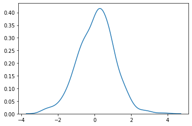
randn

backward compatibility with Matlab

takes dimensions as individual parameters

randn (n) returns a 1D ndarray

randn (3)

array([-0.69781929,  0.76250905, -0.00100293])

randn (m, n) returns a 2D (m x n) ndarray

randn (3, 2)

array([[ 0.01257397, -1.09267948],
       [ 0.43461778, -0.9010176 ],
       [ 0.94876503, -0.06544939]])

randn (i, j, k) returns a 3D (i x j x k) ndarray

randn (2, 3, 4)

array([[[-0.18420962, -2.80150569, -1.94776301,  0.58616938],
        [-0.16765517,  0.0843139 ,  0.88771571,  0.05693744],
        [ 0.88764414, -0.92584994,  0.96424221,  2.3480603 ]],

       [[-0.14195735, -0.03706071,  0.19416724, -1.05178575],
        [-0.66259882, -1.4020511 ,  0.87980418, -0.7594163 ],
        [-0.07895493,  0.68616642, -1.58868401,  1.62971673]]])

plot

sns.kdeplot (randn (500))
plt.show ()

png

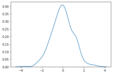
standard_normal

NumPy-centric

takes dimensions as a tuple

This allows other parameters like dtype and order to be passed to the function as well.

standard_normal ((m, n)) returns a 2D (m x n) ndarray

standard_normal ((2, 4))

array([[-1.86646271, -0.19924265,  1.13467334, -0.17763385],
       [-0.21805904, -0.47804114,  0.5908614 ,  1.49768637]])

plot

sns.kdeplot (standard_normal (500))
plt.show ()

png

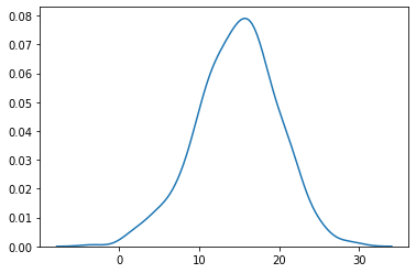
ii. np.random.normal

Generic Normal Distribution

mean: loc =
variance: scale =

NumPy-centric

takes dimensions as a tuple

This allows other parameters like loc and scale to be passed to the function as well.

normal (loc = , scale = , (m, n)) returns a 2D (m x n) ndarray with values having ‘loc’ as mean, and ‘scale’ as variance

normal (loc=15.0, scale=5.0, size=(2,3))

array([[ 7.8948123 ,  4.39815973,  9.39660432],
       [20.40527397, 19.64774283,  9.2247971 ]])

plot

sns.kdeplot (normal (loc = 15.0, scale = 5.0, size = 500))
plt.show ()

png

iii. np.random.seed and np.random.RandomState

https://stackoverflow.com/questions/5836335/consistently-create-same-random-numpy-array/5837352#5837352

A. Imports

B. Preliminaries

1. row vector, column vector, and matrix

2. np.zeros, np.ones, and np.full

numerical arrays

boolean arrays

any-type arrays

3. np.arange, and np.linspace

4. Structured arrays and Field Access

C. Array Properties

shape

size

number of dimensions

D. Array Broadcasting

1. Introduction

an example

Rules of Broadcasting

Intuition

an example

2. Inserting Size-1 Dimensions into An Array

using reshape

using np.newaxis

3. Using size-1 dimension to make arrays broadcasting compatible

E. Indexing

1. Selection Object

2. Kinds of indexing

2.1 basic slicing

2.1.1. selection object is integers or tuple

2.1.2. selection object is a slice object

2.1.3. selection object is a tuple of integers and slice objects

2.1.4. selection object is a tuple of Ellipsis and slice objects

2.1.5. selection object is a tuple of Ellipsis and integers

2.1.6. selection object is the newaxis object

2.1.7 Basic slicing extends Python’s basic concept of slicing to N dimensions.

2.2 advanced indexing

2.2.1 introduction

2.2.2 integer array indexing

2.2.3 boolean array indexing

ndarray.nonzero ()

ndarray [condition]

2.3 field access

3. flat iterator indexing

F. Vectorized Operations

a. Introduction

1. data

2. example of operations on entries of a single array

square - this is a binary operation : x ** y

np.sqrt (ndarray)

3. mathematical operations performed between two arrays are designed to act on the corresponding pairs of entries between the two arrays

+ operator

* operator

4. Operate on sequences of numbers

sum

b. Taxonomy of Operations

i. Mathematical Operations

1. Unary Functions: f (x)

np.sqrt (ndarray)

np.log (ndarray) - ln (x)

np.exp (ndarray) - e^x

2. Binary Functions: f (x, y)

+ operator

square - this is a binary operation : x ** y and np.power - one operand is a scalar

3. functions that operate on sequence of numbers: f ({x_i} i = 0..n-1)

np.mean

np.median

np.var - variance

np.std - standard deviation

np.max - see binary function ‘np.maximum’ for array of maximum elements among corresponding elements of the two arrays

np.min - minimum element of the array

np.argmax - index (sequential) of the maximum element of the array

np.argmin

np.sum

3.1 np.func (ndarray, axis = )

ii. Logical Operations

Binary operations

Sequence operations

c. Performance of Vectorized Operations

G. Linear Algebra

H. Random Sampling from Distributions

i. np.random.randn and np.random.standard_normal

square - this is a binary operation : x y and np.power - one operand is a scalar**